Static Safety Stock Is a Guess. DDMRP Buffers Are a System.

Traditional MRP calculates safety stock once, reviews it quarterly (if at all), and hopes it holds. When demand spikes, you stock out. When demand drops, you sit on excess. The buffer never adapts because it was never designed to.

DDMRP (Demand Driven Material Requirements Planning) replaces this with dynamic buffers — inventory positions that are calculated from actual demand patterns, automatically adjust to changing conditions, and generate replenishment signals based on real consumption rather than forecast projections.

This post explains exactly how DDMRP buffer management works: the zone structure, the formulas, the dynamic adjustment mechanism, and the replenishment logic. Every calculation is implemented in R with a realistic dataset of 8 electronic components.

The Three Buffer Zones

A DDMRP buffer is divided into three color-coded zones, each with a distinct purpose:

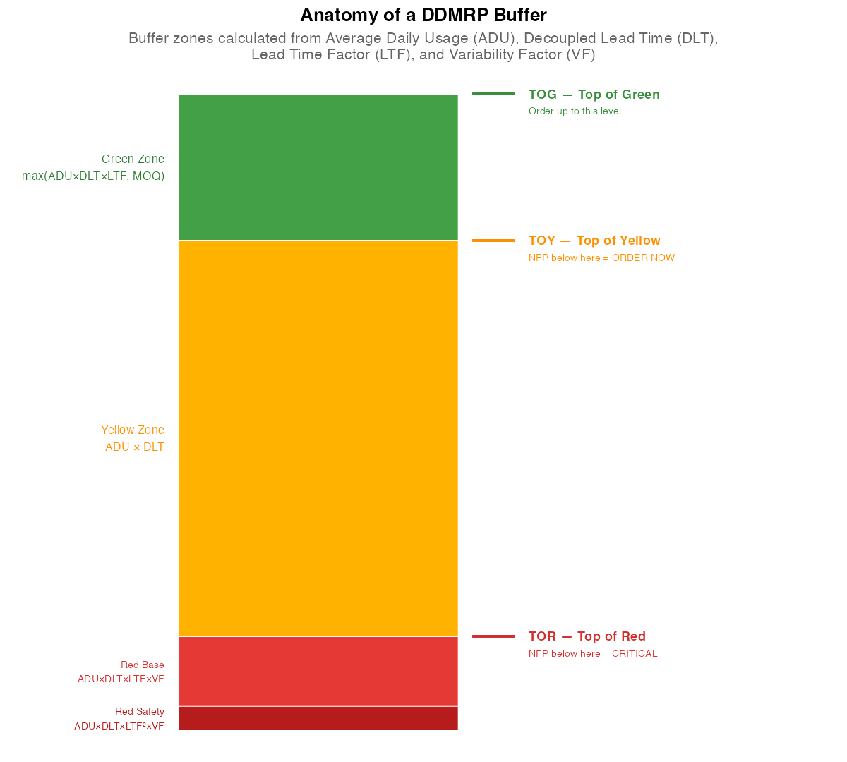
Red Zone (Bottom) — The safety zone. If the Net Flow Position drops into red, the item is at risk of stockout. The red zone itself has two parts:

• Red Base = ADU x DLT x Lead Time Factor x Variability Factor
• Red Safety = Red Base x Lead Time Factor

Items with longer lead times or higher variability get larger red zones. This is not arbitrary padding — it is a calculated protection level based on measured supply and demand characteristics.

Yellow Zone (Middle) — The order cycle zone. This represents the average consumption during one replenishment lead time:

• Yellow Zone = ADU x DLT

When the Net Flow Position drops below the Top of Yellow, a replenishment order is triggered. The yellow zone is the "normal operating range" — inventory should fluctuate within this zone during routine operations.

Green Zone (Top) — The order frequency and minimum order zone. It determines the minimum order size and prevents over-ordering:

• Green Zone = max(ADU x DLT x Lead Time Factor, Minimum Order Quantity, Imposed Order Cycle)

The green zone ensures that replenishment orders are economically sensible — you do not order 5 units when the minimum order quantity is 500.

Key terms:

• ADU = Average Daily Usage (rolling average of actual consumption)
• DLT = Decoupled Lead Time (lead time from the nearest upstream buffer)
• TOR = Top of Red (red zone ceiling)
• TOY = Top of Yellow = TOR + Yellow Zone (the reorder trigger point)
• TOG = Top of Green = TOY + Green Zone (the order-up-to level)

Calculating Buffers in R

We model 8 electronic components with realistic parameters — each has different demand rates, lead times, variability profiles, and minimum order quantities:

library(dplyr)

skus <- data.frame(
  sku       = c("PCB-100","DSP-200","BAT-300","HSG-400",
                "CAM-500","CHG-600","SPK-700","ANT-800"),
  adu       = c(45, 40, 60, 50, 35, 55, 42, 38),
  dlt       = c(12, 18, 8, 10, 20, 6, 9, 15),
  lt_factor = c(0.35, 0.40, 0.30, 0.30, 0.45, 0.25, 0.30, 0.40),
  var_factor= c(0.50, 0.60, 0.40, 0.35, 0.55, 0.30, 0.40, 0.55),
  moq       = c(200, 150, 500, 300, 100, 1000, 200, 100),
  on_hand   = c(380, 120, 850, 520, 95, 1200, 280, 60),
  on_order  = c(500, 400, 0, 300, 350, 0, 200, 0),
  qual_demand = c(210, 195, 180, 240, 175, 165, 130, 190)
)

skus <- skus %>% mutate(
  red_base    = round(adu * dlt * lt_factor * var_factor),
  red_safety  = round(red_base * lt_factor),
  red_zone    = red_base + red_safety,
  yellow_zone = round(adu * dlt),
  green_zone  = pmax(round(adu * dlt * lt_factor), moq),
  tor = red_zone,
  toy = red_zone + yellow_zone,
  tog = red_zone + yellow_zone + green_zone,
  nfp = on_hand + on_order - qual_demand,
  status = case_when(
    nfp <= tor ~ "Red",
    nfp <= toy ~ "Yellow",
    TRUE       ~ "Green"
  ),
  order_qty = ifelse(nfp < toy, tog - nfp, 0)
)

      sku adu dlt red_zone yellow_zone green_zone  tor  toy   tog   nfp status order_qty
  PCB-100  45  12      127         540        200  127  667   867   670  Green         0
  DSP-200  40  18      242         720        288  242  962  1250   325 Yellow       925
  BAT-300  60   8       75         480        500   75  555  1055   670  Green         0
  HSG-400  50  10       68         500        300   68  568   868   580  Green         0
  CAM-500  35  20      251         700        315  251  951  1266   270 Yellow       996
  CHG-600  55   6       31         330       1000   31  361  1361  1035  Green         0
  SPK-700  42   9       59         378        200   59  437   637   350 Yellow       287
  ANT-800  38  15      175         570        228  175  745   973  -130    Red      1103

The results tell a clear story. Four SKUs are healthy (green), three need replenishment orders (yellow), and one — ANT-800 — is in critical condition with a negative Net Flow Position of -130.

The Net Flow Position Equation

The Net Flow Position (NFP) is the central metric in DDMRP. It replaces MRP’s projected available balance with a simpler, more responsive calculation:

NFP = On-Hand + On-Order – Qualified Demand

• On-Hand: Physical inventory in the warehouse right now
• On-Order: Open purchase orders and production orders not yet received
• Qualified Demand: Actual demand that is due within the demand horizon (typically qualified sales orders, not forecasts)

The NFP determines what action to take:

• NFP above TOY → No action. Buffer is healthy.
• NFP between TOR and TOY → Generate a replenishment order for (TOG – NFP) units.
• NFP below TOR → Critical. Expedite existing orders and generate emergency replenishment.

Visualizing Buffer Status

The buffer overview shows all 8 SKUs with their zone structure and current NFP position:

library(ggplot2)
library(tidyr)

buffer_long <- skus %>%
  select(sku, red_zone, yellow_zone, green_zone) %>%
  pivot_longer(cols = c(red_zone, yellow_zone, green_zone),
               names_to = "zone", values_to = "size")

ggplot() +
  geom_col(data = buffer_long,
           aes(x = sku, y = size, fill = zone), width = 0.6) +
  geom_point(data = skus, aes(x = sku, y = nfp),
             shape = 18, size = 5, color = "black") +
  scale_fill_manual(values = c("red_zone" = "#D32F2F",
                                "yellow_zone" = "#FFA000",
                                "green_zone" = "#388E3C"))

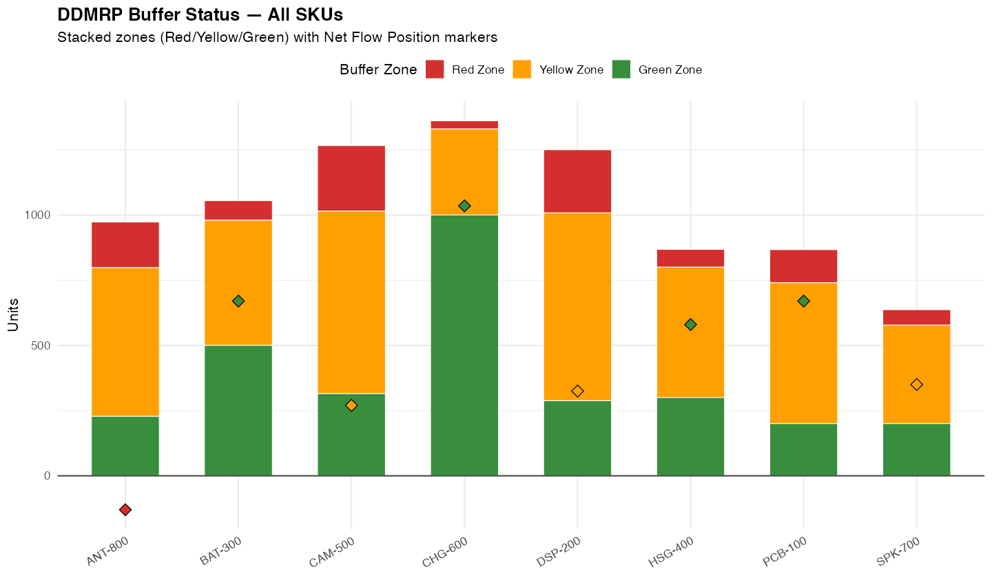
The diamond markers show where each SKU’s NFP sits within its buffer. ANT-800’s marker is below the bar entirely — its NFP is negative, meaning qualified demand exceeds available supply. DSP-200 and CAM-500 have NFPs in the yellow zone, triggering replenishment. The remaining four are comfortably in green.

A horizontal view makes the zone penetration easier to compare across SKUs:

ggplot(skus) +
  geom_segment(aes(x = 0, xend = tor, y = reorder(sku, nfp/tog),
                   yend = reorder(sku, nfp/tog)),
               color = "#FFCDD2", linewidth = 12) +
  geom_segment(aes(x = tor, xend = toy, y = reorder(sku, nfp/tog),
                   yend = reorder(sku, nfp/tog)),
               color = "#FFF9C4", linewidth = 12) +
  geom_segment(aes(x = toy, xend = tog, y = reorder(sku, nfp/tog),
                   yend = reorder(sku, nfp/tog)),
               color = "#C8E6C9", linewidth = 12) +
  geom_point(aes(x = nfp, y = reorder(sku, nfp/tog)),
             shape = "|", size = 8, color = "black")

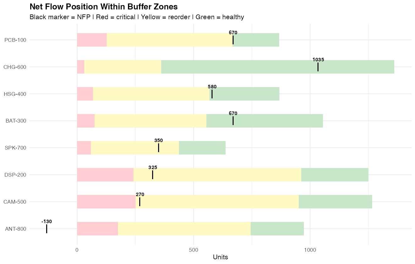
Sorted by buffer penetration, the most critical items float to the bottom. ANT-800 is off the chart to the left (negative NFP). This is the view a planner checks every morning — it tells you exactly which items need attention and how urgent each one is.

Dynamic Adjustment: Buffers That Breathe

This is where DDMRP fundamentally differs from static safety stock. Buffers are not fixed numbers — they adjust based on Demand Adjustment Factors (DAF).

When a planned event changes expected demand — a seasonal peak, a product launch, a major customer promotion — the planner applies a DAF to the ADU. A DAF of 1.4 means demand is expected to increase by 40%. The buffer zones recalculate automatically:

# Normal ADU for PCB-100: 45 units/day
# Seasonal peak DAF: 1.4 → adjusted ADU: 63 units/day
# All buffer zones expand proportionally

pcb_normal <- data.frame(
  red_zone    = 127, yellow_zone = 540, green_zone = 200)   # TOG = 867
pcb_peak   <- data.frame(
  red_zone    = 249, yellow_zone = 756, green_zone = 265)   # TOG = 1270

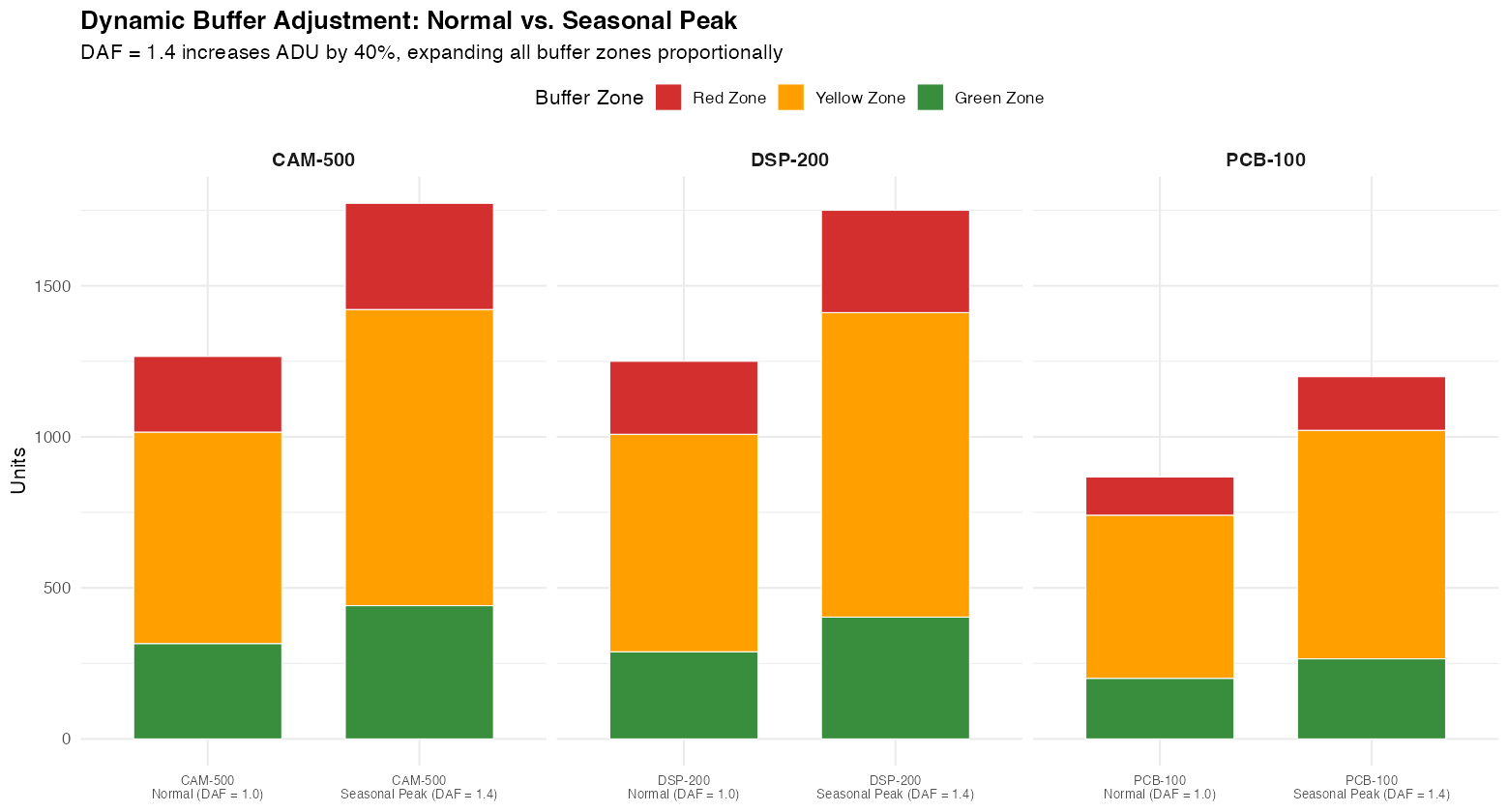
The visual difference is striking. During a seasonal peak (DAF = 1.4), every zone grows — the red zone expands to provide more safety, the yellow zone extends to cover the higher daily consumption, and the green zone adjusts the minimum order size upward.

When the peak passes, the DAF returns to 1.0 and the buffers contract. No manual safety stock review needed. No quarterly rebalancing meetings. The system breathes with demand.

This is also where the planner adds value. The DAF is not automatic — it is a deliberate planning input based on market intelligence, customer forecasts, and seasonal knowledge. DDMRP automates the buffer math but relies on human judgment for demand signals.

Net Flow Position Over Time

To see how buffer management works in practice, we simulate 30 days of operations for PCB-100. Daily demand fluctuates around the ADU of 45 units. Replenishment orders are triggered whenever the NFP drops below TOY (667 units) and sized to bring the NFP back up to TOG (867 units):

# Simulation loop (simplified)
for (d in 1:30) {
  oh <- oh + arriving_orders[d] - daily_demand[d]
  nfp <- oh + future_on_order - qualified_demand_3day

  if (nfp < toy) {
    order_qty <- max(tog - nfp, moq)
    place_order(order_qty, arrival = d + dlt)
  }
}

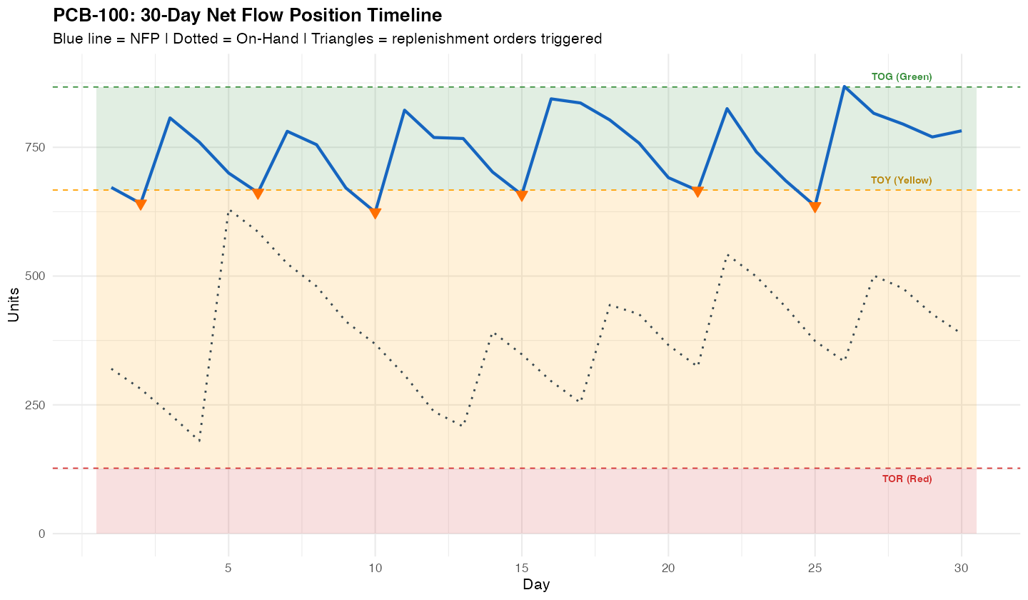
The blue line shows the NFP fluctuating within the buffer zones. When it crosses the TOY threshold (yellow dashed line), a replenishment order is triggered (orange triangle). The order arrives after the 12-day decoupled lead time, and the NFP recovers.

Key observations from the simulation:

• The NFP stays mostly in the green and upper yellow zones — the buffer is properly sized for normal demand variation.
• Replenishment orders are triggered by actual consumption, not by a forecast schedule. The timing adapts to real conditions.
• The on-hand line (dotted) diverges from the NFP when open orders exist. On-hand can be low while NFP is healthy because incoming orders are accounted for.
• The system self-corrects. A demand spike draws down the buffer, triggers a replenishment, and the buffer refills. No planner intervention needed for routine fluctuations.

Replenishment Priorities

When multiple SKUs need replenishment simultaneously, buffer penetration determines priority. Higher penetration means the NFP has dropped deeper into the buffer — and deeper means more urgent:

reorder_skus <- skus %>%
  filter(order_qty > 0) %>%
  mutate(penetration = round((1 - nfp / tog) * 100, 1)) %>%
  arrange(desc(penetration))

ggplot(reorder_skus, aes(x = reorder(sku, penetration),
                          y = penetration, fill = urgency)) +
  geom_col(width = 0.6) +
  coord_flip()

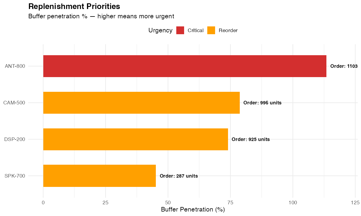
ANT-800 is at over 100% penetration (NFP is negative) — this is a critical expedite situation. CAM-500 and DSP-200 are in the yellow zone and need standard replenishment orders. SPK-700 just crossed into yellow — it can wait a day but should be ordered soon.

This priority board replaces the MRP exception message list. Instead of hundreds of undifferentiated action messages, you get a ranked list with clear visual urgency. Planners focus on red first, then yellow. Green items need no attention.

The Five Components of DDMRP Buffer Management

To summarize the system:

1. Strategic Buffer Positioning — Not every item gets a buffer. Buffers are placed at decoupling points — locations in the BOM or supply chain where you want to break the dependency chain and absorb variability. Positioning is a design decision.

2. Buffer Profiling and Sizing — Items are grouped into buffer profiles based on lead time range, variability category, and item type (manufactured, purchased, distributed). Each profile has standardized lead time factors and variability factors. Buffer zones are calculated from ADU, DLT, and these factors.

3. Dynamic Adjustment — Demand Adjustment Factors (DAF) scale the ADU up or down for planned events. Lead Time Adjustment Factors handle known supply changes. Buffers recalculate automatically when factors change.

4. Demand-Driven Planning — The Net Flow Position equation (On-Hand + On-Order – Qualified Demand) drives replenishment. Orders are generated when NFP drops below TOY, sized to bring NFP back to TOG. No forecast explosion. No MRP nervousness.

5. Visible Execution — Buffer status is communicated through color: red means act now, yellow means order, green means healthy. Priorities are set by penetration depth, not by planner judgment or first-come-first-served.

Why This Works Better Than Static Safety Stock

Traditional safety stock has three fundamental problems that DDMRP buffers solve:

Safety stock does not know why it exists. It is a number in a field. A DDMRP buffer is a structured system with distinct zones that serve different purposes — safety, replenishment cycle, and order sizing.

Safety stock does not adjust. It sits at the same level whether demand doubles or halves. DDMRP buffers adjust dynamically through DAF, and the ADU itself rolls forward as actual demand accumulates.

Safety stock does not prioritize. When 200 items need attention, MRP gives you 200 exception messages with equal urgency. DDMRP gives you a color-coded priority board ranked by buffer penetration. Planners work the red items first and ignore the green ones.

The result is less inventory, better service levels, and planners who spend their time on exceptions rather than routine transactions.

Interactive Dashboard

See all of these concepts in a single operational view: DDMRP Dynamic Buffer Management Dashboard — featuring live buffer zone visualization, net flow position timeline, buffer penetration heat map, replenishment signal board, and dynamic adjustment demo for all 8 SKUs.