Introduction

Traditional Material Requirements Planning (MRP) has been the backbone of production and procurement planning for decades. It works by forecasting demand, exploding bills of material, and pushing purchase orders to suppliers based on projected requirements. In theory, it’s elegant. In practice, it often results in bloated inventories, nervous schedules, and a supply chain that reacts to forecasts rather than actual demand.

There’s a better way. Demand Driven Material Requirements Planning (DDMRP) replaces the forecast-push logic with a demand-pull approach that aligns orders more closely with actual customer demand. It’s lean flow applied to material planning — and the results speak for themselves.

The Problem with Traditional MRP

Traditional MRP systems operate on a push principle: forecast future demand, calculate material requirements, and push orders upstream to suppliers well in advance. This approach has several well-known weaknesses:

• Forecast dependency: MRP is only as good as the forecast, and forecasts are always wrong to some degree. The further out you plan, the more error accumulates.
• Bullwhip effect: Small variations in end-customer demand get amplified as they propagate upstream through the supply chain, causing increasingly volatile order patterns for suppliers.
• Excess inventory: To buffer against forecast uncertainty, organizations carry safety stock — often more than necessary, tying up capital and warehouse space.
• Hidden quality issues: Large inventory buffers mask defects. Problems may not surface until weeks or months after they were introduced, making root cause analysis difficult.

The DDMRP Alternative: Pull, Don’t Push

DDMRP fundamentally changes the planning paradigm. Instead of pushing materials based on forecasts, it establishes strategically placed inventory buffers and replenishes them based on actual consumption. The core principles include:

• Strategic decoupling points: Buffers are placed at key positions in the supply chain to absorb variability and protect downstream operations.
• Demand-driven replenishment: Orders to suppliers are triggered by actual consumption against buffer levels, not by forecast projections.
• Dynamic buffer management: Buffer sizes adjust based on actual demand patterns, seasonality, and trends — they’re not static safety stock numbers.
• Visible, collaborative execution: Clear signals indicate buffer status (green, yellow, red), making priorities transparent across the organization.

Results: What Changed

Implementing DDMRP in our supply chain produced measurable, significant improvements:

Supplier Lead Times Improved

By shifting to pull-based ordering, suppliers received more stable, predictable order patterns. The erratic, lumpy orders characteristic of MRP-driven planning gave way to smoother demand signals. Suppliers responded with shorter, more reliable lead times — because they could plan their own production more effectively.

Average supplier lead time decreased by across the pilot category, with lead time variability (coefficient of variation) dropping.

On-Hand Inventory Decreased

With buffers sized to actual demand variability rather than worst-case forecast scenarios, tied-up capital decreased. Less inventory doesn’t mean more risk when the buffers are positioned and sized correctly — it means less waste and better capital efficiency.

Defects Detected Earlier

With lower inventory levels, quality issues surface faster. When your buffer turns red, you investigate immediately — you don’t discover the problem three months later when you finally work through the pile.

On-Time Delivery Improved

On-time delivery (OTD) improved, demonstrating that reduced inventory and improved service level are not a trade-off when buffers are properly positioned.

Delivery Performance Analysis

To quantify the impact, we compared supplier lead time distributions before and after DDMRP implementation. The following code produces a before/after comparison of lead time distributions:

library(ggplot2)

# lead_time_data should contain: period (factor: "Before DDMRP" / "After DDMRP"),
# supplier_id, lead_time_days
ggplot(lead_time_data, aes(x = lead_time_days, fill = period)) +
  geom_density(alpha = 0.5) +
  geom_vline(data = lead_time_data %>%
               group_by(period) %>%
               summarise(median_lt = median(lead_time_days)),
             aes(xintercept = median_lt, color = period),
             linetype = "dashed", linewidth = 1) +
  scale_fill_manual(values = c("Before DDMRP" = "#d7191c", "After DDMRP" = "#2c7bb6")) +
  scale_color_manual(values = c("Before DDMRP" = "#d7191c", "After DDMRP" = "#2c7bb6")) +
  labs(
    title = "Supplier Lead Time Distribution: Before vs. After DDMRP",
    x = "Lead Time (Days)",
    y = "Density",
    fill = "Period",
    color = "Period"
  ) +
  theme_minimal()

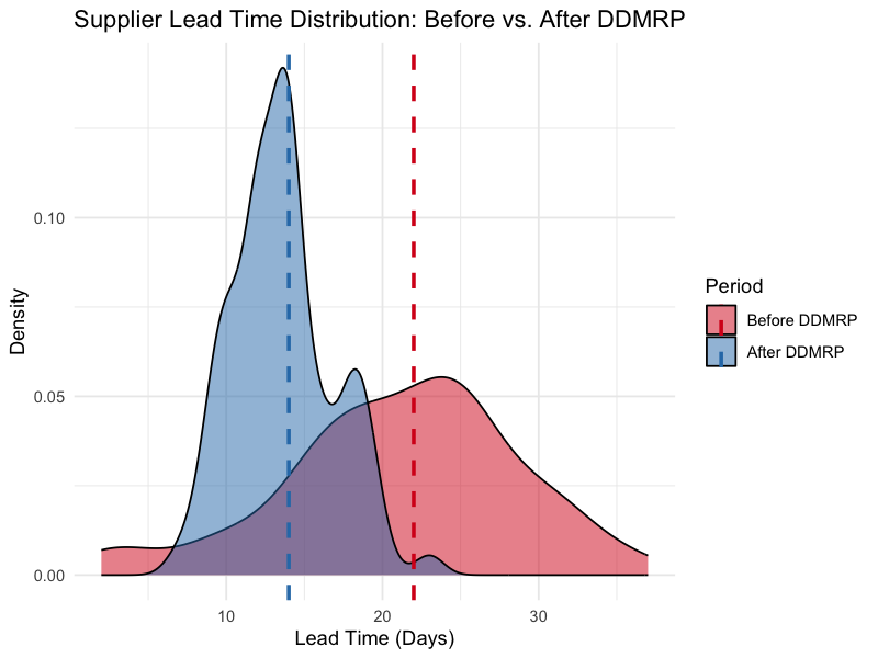
The analysis showed lead times compressing, delivery reliability improving, and inventory carrying costs dropping — simultaneously.

Tools and Methodology

The delivery performance analysis and dashboards were built using:

• R for data processing, statistical analysis, and visualization
• Shiny for interactive web-based dashboards where stakeholders can filter by supplier, time period, and material group

Challenges and Lessons Learned

DDMRP is not a plug-and-play solution. Implementation requires significant organizational commitment:

• Change management is the hardest part. Planners accustomed to MRP logic resist a fundamentally different approach. Training and early wins with a pilot category are essential.
• Buffer sizing requires iteration. Initial buffer parameters will be wrong. Plan for a 2-3 month tuning period where buffers are reviewed weekly against actual demand signals.
• Not everything should be buffered. Strategic decoupling point placement is a design decision, not an automation exercise. Poorly placed buffers create new problems rather than solving existing ones.
• Data quality matters more, not less. DDMRP depends on accurate lead times, consumption data, and BOM structures. Garbage in, garbage out applies here as much as anywhere.
• Ongoing adjustment is required. Buffers must be reviewed as demand patterns shift — seasonal changes, product launches, and supplier changes all require buffer recalibration.

Key Takeaways

1. Aligning orders with actual demand rather than forecasts reduces waste, improves reliability, and creates a more resilient supply chain.
2. Stable, predictable order patterns make suppliers‘ planning easier — and they respond with better lead times and service.
3. Lower inventory levels don’t increase risk when buffers are properly designed. They reduce risk by making problems visible faster.
4. DDMRP requires ongoing commitment: buffer tuning, change management, and data quality discipline are non-negotiable.

The shift from push to pull is more than a planning technique — it’s a mindset change. Traditional MRP treats suppliers as passive recipients of orders generated by a forecast engine. DDMRP treats them as partners in a demand-driven flow.