A Story You Already Lived Through
Remember March 2020, when you walked into a grocery store and the toilet paper aisle looked like a post-apocalyptic movie set? Retail sales spiked 734% in a single day. Stores across the country ran dry. Social media was full of people posing with their hoarded stacks like trophies.
Here’s the thing: nobody’s bathroom habits changed. Babies still used the same number of diapers. Adults didn’t suddenly start using three times more toilet paper. Actual consumption barely budged. What did happen was a textbook case of the bullwhip effect — a phenomenon where a modest tremor in consumer demand turns into an earthquake by the time it reaches the upstream end of the supply chain.
And this wasn’t the first time. The same pattern shows up everywhere from Pampers diapers to semiconductors to lumber. It has cost individual companies billions and entire industries hundreds of billions. The bullwhip effect is arguably the most expensive recurring mistake in supply chain management.
The good news? It’s quantifiable, simulatable, and — to a meaningful degree — tameable. Let’s dig in.
What Exactly Is the Bullwhip Effect?
The name comes from the physics of a whip: a small flick of the wrist at the handle produces increasingly larger waves traveling toward the tip. In a supply chain, the "handle" is end-consumer demand and the "tip" is the raw-material supplier several echelons upstream.
Formally, we measure it as a variance ratio:
BWE = Var(Orders) / Var(Demand)
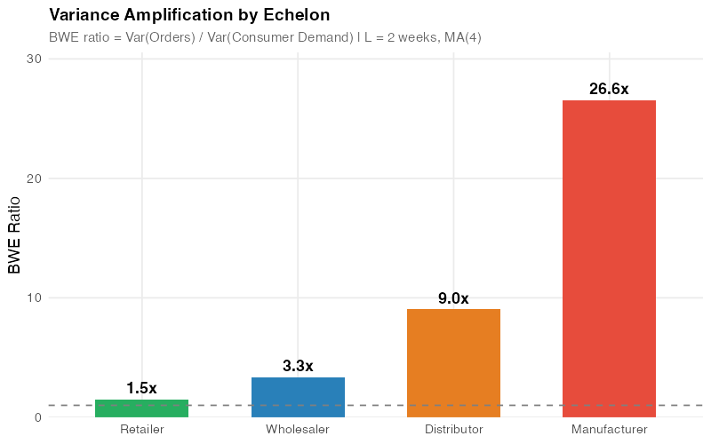
A ratio of 1.0 means orders perfectly mirror demand — no amplification. Anything above 1.0 means the signal is getting distorted, and the higher the number, the worse the distortion. In practice, ratios of 2x to 5x per echelon are common, and they compound multiplicatively across the chain.
So if you have four echelons (retailer, wholesaler, distributor, manufacturer) and each one amplifies variance by a factor of 2, the manufacturer experiences:
2 x 2 x 2 x 2 = 16 times the variance of actual consumer demand.
A 5% wobble at the cash register becomes an 80% swing at the factory floor. That’s not a rounding error — that’s the difference between running overtime and laying people off.
A Brief History: From Forrester to Pampers
Jay Forrester at MIT first described demand amplification in 1961 in his book Industrial Dynamics. He used system dynamics models to show how information delays and feedback loops in industrial supply chains create self-reinforcing oscillations. He called it the "Forrester Effect," which frankly sounds like a spy thriller.
The more evocative name came from Procter & Gamble in the 1990s. P&G logistics executives studied order patterns for Pampers diapers and noticed something paradoxical: baby diaper consumption is about as stable as demand gets (babies are remarkably consistent in this regard), yet order variability increased at every echelon. Retailer orders to wholesalers fluctuated. Wholesaler orders to distributors fluctuated more. And P&G’s own orders to raw material suppliers like 3M fluctuated the most.
Each echelon was interpreting the previous level’s orders as a demand signal and adding its own safety buffer, forecast adjustment, and batch sizing on top. The result was an amplification cascade that the P&G team aptly named the "bullwhip effect."
In 1997, Stanford researchers Hau Lee, V. Padmanabhan, and Seungjin Whang formalized the concept in two landmark papers and identified four root causes. Three years later, Chen, Drezner, Ryan, and Simchi-Levi (2000) provided the first rigorous mathematical lower bounds for the variance amplification ratio. These formulas are the foundation of the simulation we’ll build below.
The Four Root Causes
Lee, Padmanabhan, and Whang (1997) identified four mechanisms that drive the bullwhip effect. Understanding them is important because each one has a different countermeasure — there is no single silver bullet.
1. Demand Signal Processing
Every echelon creates its own demand forecast based on the orders it receives, not on actual end-consumer demand. When a retailer sees a small uptick and raises its safety stock, the wholesaler sees an inflated order, adjusts its own forecast, adds more safety stock, and orders even more. Each echelon compounds the distortion.
The key insight: longer lead times make this worse because they require more safety stock to cover a longer uncertain horizon.
2. Order Batching
Companies accumulate demand and order periodically — weekly, biweekly, monthly — rather than continuously. This creates spiky, lumpy order patterns even when the underlying demand is smooth. If multiple retailers batch their orders on the same cycle (say, every Monday), the wholesaler sees a massive spike followed by silence. This has nothing to do with actual demand and everything to do with ordering calendars and full-truckload economics.
3. Price Fluctuations and Forward Buying
Trade promotions, quantity discounts, and end-of-quarter fire sales incentivize forward buying — purchasing more than you need while prices are low. This creates artificial demand spikes that have zero relationship to actual consumption. The post-promotion demand crater is just as damaging as the spike itself.
4. Rationing and Shortage Gaming
When a product is scarce, suppliers often allocate based on order quantities. Customers learn this and inflate their orders to game the allocation — so-called "phantom orders." When supply normalizes, they cancel the excess, and the supplier is left holding a mountain of unneeded inventory.
HP learned this the hard way with the LaserJet III: resellers inflated orders during a shortage, then cancelled en masse when supply recovered, leaving HP with millions in excess inventory. Cisco’s experience during the dot-com bust was even more dramatic — a $2.2 billion inventory write-down from order cancellations.
The Math: How Bad Can It Get?
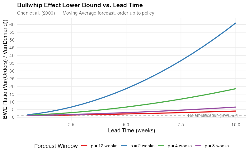
Chen et al. (2000) derived a lower bound for variance amplification when a retailer uses a simple moving average (MA) forecast with p demand observations and an order-up-to policy with lead time L:
Var(q) / Var(D) >= 1 + (2L / p) + (2L^2 / p^2)
This formula is elegant and terrifying in equal measure. Notice that amplification grows with the square of lead time. Cutting a 4-week lead time in half — to 2 weeks — doesn’t just halve the excess variance, it slashes it by 63% (from a BWE of 5.0 down to 2.5). This is why lead time reduction is the single most powerful lever in your toolkit.
Here’s what the numbers look like for a 4-week moving average:
| Lead Time (weeks) | BWE Lower Bound | Amplification |
|---|---|---|
| 1 | 1.63 | +63% |
| 2 | 2.50 | +150% |
| 3 | 3.63 | +263% |
| 4 | 5.00 | +400% |
| 6 | 8.50 | +750% |
| 8 | 13.00 | +1200% |
And remember — these are lower bounds. Actual amplification is typically worse. Also remember that this is per echelon. In a 4-tier chain where each echelon has a 2-week lead time (BWE of 2.5), the manufacturer faces a compound amplification of 2.5^4 = 39 times the consumer demand variance.
Let that sink in.
Simulating the Bullwhip: A 4-Tier Supply Chain in R
Theory is useful, but nothing drives the point home like watching the bullwhip effect unfold in a simulation. Below, we simulate a 4-tier supply chain — consumer, retailer, wholesaler, distributor, manufacturer — where each echelon uses a moving average forecast and an order-up-to inventory policy.
The consumer demand is deliberately boring: a stationary process with a mean of 100 units per week, a small standard deviation, and a single modest 10% step-up at week 25. Nothing dramatic. Just the kind of demand variation you’d see on any given Tuesday.
What happens upstream is anything but boring.
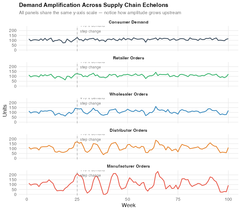
The chart tells the story: that quiet 10% step-up at the consumer level turns into swings of 40-60% at the manufacturer level, with overshoot, oscillation, and a recovery period that stretches far longer than the original demand event. The manufacturer has no idea whether they should be ramping up production or shutting down lines.
Real-World Damage: The Numbers Are Staggering
The bullwhip effect isn’t an academic curiosity. It has caused some of the most expensive supply chain failures in business history.
The COVID toilet paper crisis (2020): Consumer demand rose 20-40%. Retailer orders doubled. Distributor orders tripled. 70% of U.S. grocery stores ran out of stock despite manufacturers running at full capacity. The "shortage" was entirely a demand-signal distortion.
The semiconductor crisis (2020-2023): Auto manufacturers cancelled chip orders in early 2020 when car sales dropped. When demand recovered, chips were allocated to consumer electronics. The shortage affected 169+ industries. The U.S. auto industry alone lost an estimated $240 billion in 2021. Ford cut production by 50% in Q2 2021. GM estimated a $1.5-2 billion cost impact. The average car price jumped more than 15% in under two years.
The lumber price explosion (2020-2021): Prices surged approximately 530% from April 2020 to May 2021, peaking at $1,630 per 1,000 board feet (vs. ~$260 pre-pandemic). This added an estimated $24,000 to the cost of a new single-family home. When the bullwhip snapped back, prices crashed almost as fast as they rose — classic overshoot and correction.
Cisco (2001): During the dot-com boom, customers double- and triple-ordered networking equipment. When the bubble burst, order cancellations left Cisco with a $2.2 billion inventory write-down. That’s roughly $3.4 billion in today’s dollars.
Taming the Whip: What Actually Works
The bad news: a study of 15,000 firms over 36 years found no significant decrease in the bullwhip effect over time. Despite decades of awareness, tools, and technology, the problem persists. The bullwhip effect is fundamentally a human and structural problem, not just a data problem.
The good news: the math tells us exactly which levers matter most, and some interventions produce dramatic results.
Lead Time Reduction: The Most Powerful Lever
The Chen et al. formula shows variance amplification grows with L^2. Findings from the MIT Beer Game confirm it: cutting order-to-delivery time in half reduces supply chain fluctuations by 80%. No other single intervention comes close.
Practical approaches: supplier co-location, pre-positioned inventory, faster transportation modes, streamlined order processing.
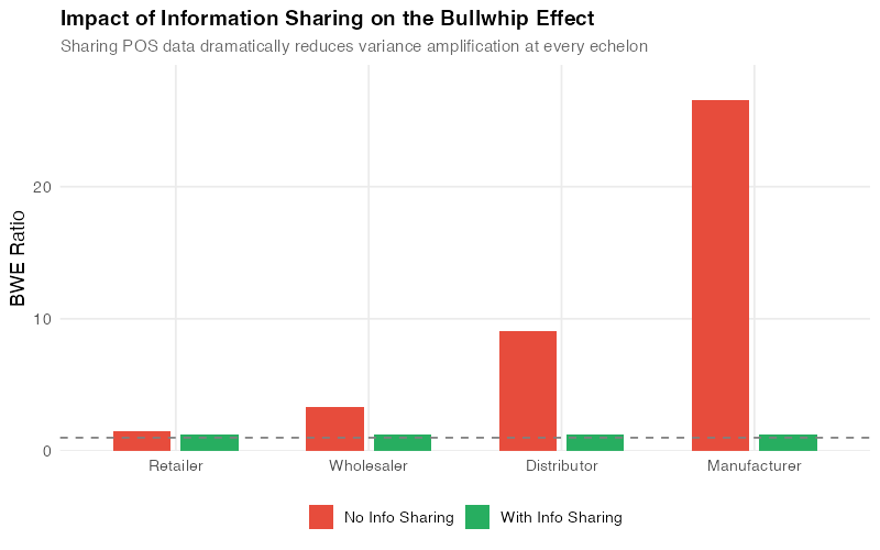
Information Sharing: See the Real Signal
When every echelon reacts to the orders it receives rather than actual consumer demand, distortion is inevitable. Sharing point-of-sale data across the entire chain lets everyone work from the same demand signal.
Walmart’s Retail Link system transmits POS data from every store to headquarters multiple times daily. Suppliers see actual consumer purchases, not amplified orders. The result: an estimated 10-15% inventory reduction across the network.
Vendor-Managed Inventory (VMI)
When the supplier manages inventory at the customer’s location, you eliminate the customer’s forecasting and ordering distortions entirely. Disney and Towill (2003) demonstrated that VMI can reduce the bullwhip effect by 50%.
Every Day Low Pricing (EDLP)
Eliminating deep promotional discounts removes the forward-buying incentive. No price spikes means no artificial demand spikes. Walmart pioneered this approach, and it works.
Allocation Based on Past Sales
During shortages, allocate supply based on verified historical sales — not current order quantities. This removes the incentive for phantom orders. Several semiconductor companies adopted this during the 2020-2023 chip shortage.
The Forecasting Trade-Off
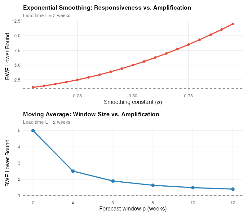
There’s an inherent tension in forecasting that directly affects the bullwhip effect. The Chen et al. formula for exponential smoothing is:
Var(q) / Var(D) >= 1 + (2L * alpha) + (2L^2 * alpha^2)
A high smoothing constant (alpha close to 1) makes your forecast responsive to recent changes but amplifies the bullwhip. A low alpha smooths the signal and reduces amplification but makes you slow to react to genuine demand shifts. Moving averages with longer windows (larger p) behave similarly — more smoothing, less amplification, slower response.
This trade-off is fundamental: you cannot simultaneously be maximally responsive and minimally amplifying. The best you can do is find the sweet spot for your specific supply chain, and the R simulation below lets you explore exactly that.
What Modern Tools Bring to the Table
AI-driven demand sensing uses POS data, weather patterns, social media trends, and geopolitical signals to forecast demand with more precision than traditional statistical methods. Deep reinforcement learning agents are being trained to optimize ordering policies that specifically minimize bullwhip amplification.
Digital twins — real-time virtual replicas of supply chains — allow you to simulate ordering policies before deploying them. You can test how a change in lead time, batch size, or information sharing policy would affect variance amplification without putting real inventory at risk.
But technology alone won’t save you. The bullwhip effect is driven as much by organizational incentives, batching habits, and procurement policies as by forecasting accuracy. The firms that tame it are the ones that combine better data with better process design.
Interactive Dashboard
Explore the data yourself — adjust lead times, forecast windows, smoothing constants, and the number of supply chain echelons to see how the bullwhip effect responds in real time.
Interactive Dashboard
Explore the data yourself — adjust parameters and see the results update in real time.
Your Next Steps
The bullwhip effect is quantifiable, and that means it’s manageable. Here’s what you can do this week:
-
Measure your BWE ratio. Pull 12 months of order data and compute Var(Orders) / Var(Demand) at each echelon. If you’re above 2.0, you have a significant amplification problem. The R code below gives you everything you need to run this analysis on your own data.
-
Map your lead times. Identify the longest lead times in your supply chain. The math says reducing them is the highest-ROI intervention. Even shaving one week off a 4-week lead time drops the theoretical lower bound from 5.0 to 3.6 — a 28% improvement.
-
Audit your ordering policies. Are you batching orders weekly when daily would be feasible? Are promotions creating artificial demand spikes? Are shortage allocations based on current orders (incentivizing gaming) or historical sales?
-
Share demand data upstream. If your suppliers are forecasting based on your orders rather than your actual consumption, you are the whip handle. Share POS or consumption data, and you’ll smooth the signal for everyone upstream.
-
Run the simulation. Use the R code and the interactive dashboard to model your own supply chain parameters. Show your leadership team what a 2-week lead time reduction would mean in concrete variance and cost terms. Numbers move decisions.
Show R Code
# =============================================================================
# Bullwhip Effect Simulation and Analysis
# =============================================================================
# A complete R simulation of the bullwhip effect in a 4-tier supply chain.
# Generates all visualizations and variance analyses used in this post.
#
# Required packages: ggplot2, dplyr, tidyr, scales, patchwork
# =============================================================================

library(ggplot2)
library(dplyr)
library(tidyr)
library(scales)
library(patchwork)

# Set seed for reproducibility
set.seed(42)

# --- Theme for all plots ---
theme_bullwhip <- theme_minimal(base_size = 13) +
  theme(
    plot.title = element_text(face = "bold", size = 14),
    plot.subtitle = element_text(color = "grey40", size = 11),
    panel.grid.minor = element_blank(),
    legend.position = "bottom"
  )

# =============================================================================
# 1. BULLWHIP EFFECT FORMULAS
# =============================================================================

# Chen et al. (2000) lower bound — Moving Average
bwe_ma_lower_bound <- function(L, p) {
  1 + (2 * L / p) + (2 * L^2 / p^2)
}

# Chen et al. (2000) lower bound — Exponential Smoothing
bwe_es_lower_bound <- function(L, alpha) {
  1 + (2 * L * alpha) + (2 * L^2 * alpha^2)
}

# Basic BWE ratio from data
bwe_ratio <- function(orders, demand) {
  var(orders, na.rm = TRUE) / var(demand, na.rm = TRUE)
}

# =============================================================================
# 2. THEORETICAL BWE vs LEAD TIME (Chart 1)
# =============================================================================

lead_times <- seq(0.5, 10, by = 0.5)
forecast_windows <- c(2, 4, 8, 12)

bwe_theory <- expand.grid(L = lead_times, p = forecast_windows) %>%
  mutate(
    BWE = bwe_ma_lower_bound(L, p),
    Forecast_Window = paste0("p = ", p, " weeks")
  )

p1 <- ggplot(bwe_theory, aes(x = L, y = BWE, color = Forecast_Window)) +
  geom_line(linewidth = 1.2) +
  geom_hline(yintercept = 1, linetype = "dashed", color = "grey50") +
  annotate("text", x = 9, y = 1.3, label = "No amplification (BWE = 1)",
           color = "grey50", size = 3.5) +
  scale_color_manual(values = c("#e41a1c", "#377eb8", "#4daf4a", "#984ea3")) +
  scale_y_continuous(breaks = seq(0, 60, by = 5)) +
  labs(
    title = "Bullwhip Effect Lower Bound vs. Lead Time",
    subtitle = "Chen et al. (2000) — Moving Average forecast, order-up-to policy",
    x = "Lead Time (weeks)",
    y = "BWE Ratio (Var(Orders) / Var(Demand))",
    color = "Forecast Window"
  ) +
  theme_bullwhip

print(p1)

# =============================================================================
# 3. 4-TIER SUPPLY CHAIN SIMULATION
# =============================================================================

simulate_supply_chain <- function(
    n_periods = 100,
    base_demand = 100,
    demand_sd = 10,
    step_change = 10,        # demand increase at step_week
    step_week = 25,
    lead_time = 2,
    forecast_window = 4,
    info_sharing = FALSE     # if TRUE, all echelons see consumer demand
) {

  # Generate consumer demand: stationary with step change
  consumer_demand <- numeric(n_periods)
  for (t in 1:n_periods) {
    base <- ifelse(t >= step_week, base_demand + step_change, base_demand)
    consumer_demand[t] <- max(0, rnorm(1, mean = base, sd = demand_sd))
  }

  # Chen et al. (2000) order-up-to policy:
  #   q_t = d_t + L * (MA_t - MA_{t-1})
  # This amplifies variance while keeping the mean stable across echelons.
  compute_orders <- function(incoming, L, p) {
    n <- length(incoming)
    orders <- numeric(n)
    orders[1:(p + 1)] <- incoming[1:(p + 1)]

    for (t in (p + 2):n) {
      ma_curr <- mean(incoming[(t - p):(t - 1)])
      ma_prev <- mean(incoming[(t - p - 1):(t - 2)])
      orders[t] <- incoming[t] + L * (ma_curr - ma_prev)
      orders[t] <- max(0, orders[t])
    }
    orders
  }

  retailer <- compute_orders(consumer_demand, lead_time, forecast_window)

  if (info_sharing) {
    wholesaler  <- compute_orders(consumer_demand, lead_time, forecast_window)
    distributor <- compute_orders(consumer_demand, lead_time, forecast_window)
    manufacturer <- compute_orders(consumer_demand, lead_time, forecast_window)
  } else {
    wholesaler  <- compute_orders(retailer, lead_time, forecast_window)
    distributor <- compute_orders(wholesaler, lead_time, forecast_window)
    manufacturer <- compute_orders(distributor, lead_time, forecast_window)
  }

  data.frame(
    week = 1:n_periods,
    Consumer_Demand = consumer_demand,
    Retailer = retailer,
    Wholesaler = wholesaler,
    Distributor = distributor,
    Manufacturer = manufacturer
  )
}

# Run simulation — no information sharing
sim_no_share <- simulate_supply_chain(info_sharing = FALSE)

# Run simulation — with information sharing
sim_with_share <- simulate_supply_chain(info_sharing = TRUE)

# =============================================================================
# 4. TIME SERIES PLOT — Orders at Each Echelon (Chart 2)
# =============================================================================

sim_long <- sim_no_share %>%
  pivot_longer(
    cols = -week,
    names_to = "Echelon",
    values_to = "Units"
  ) %>%
  mutate(Echelon = factor(Echelon,
    levels = c("Consumer_Demand", "Retailer", "Wholesaler",
               "Distributor", "Manufacturer"),
    labels = c("Consumer Demand", "Retailer Orders", "Wholesaler Orders",
               "Distributor Orders", "Manufacturer Orders")
  ))

echelon_colors <- c(
  "Consumer Demand"     = "#2c3e50",
  "Retailer Orders"     = "#27ae60",
  "Wholesaler Orders"   = "#2980b9",
  "Distributor Orders"  = "#e67e22",
  "Manufacturer Orders" = "#e74c3c"
)

p2 <- ggplot(sim_long, aes(x = week, y = Units, color = Echelon)) +
  geom_line(linewidth = 0.9, alpha = 0.85) +
  geom_vline(xintercept = 25, linetype = "dashed", color = "grey40", alpha = 0.6) +
  annotate("text", x = 26, y = max(sim_no_share$Manufacturer, na.rm = TRUE) * 0.95,
           label = "+10% demand\nstep change", hjust = 0, size = 3.2, color = "grey40") +
  scale_color_manual(values = echelon_colors) +
  labs(
    title = "The Bullwhip Effect in Action",
    subtitle = "4-tier supply chain | L = 2 weeks | MA(4) forecast | 10% demand step at week 25",
    x = "Week", y = "Order Quantity (units)",
    color = NULL
  ) +
  theme_bullwhip

print(p2)

# =============================================================================
# 5. FACETED PANEL — Same data, one panel per echelon (Chart 2 alt)
# =============================================================================

p2_facet <- ggplot(sim_long,
                   aes(x = week, y = Units, color = Echelon)) +
  geom_line(linewidth = 0.8) +
  geom_vline(xintercept = 25, linetype = "dashed", color = "grey40", alpha = 0.5) +
  facet_wrap(~ Echelon, ncol = 1) +
  scale_color_manual(values = echelon_colors, guide = "none") +
  labs(
    title = "Demand Amplification Across Supply Chain Echelons",
    subtitle = "All panels share the same y-axis scale — notice how amplitude grows upstream",
    x = "Week", y = "Units"
  ) +
  theme_bullwhip +
  theme(strip.text = element_text(face = "bold"))

print(p2_facet)

# =============================================================================
# 6. VARIANCE RATIO BAR CHART (Chart 3)
# =============================================================================

# Calculate BWE ratios (use only the stabilized portion of the simulation)
stable_range <- 15:100

bwe_ratios <- data.frame(
  Echelon = c("Retailer", "Wholesaler", "Distributor", "Manufacturer"),
  BWE = c(
    bwe_ratio(sim_no_share$Retailer[stable_range],
              sim_no_share$Consumer_Demand[stable_range]),
    bwe_ratio(sim_no_share$Wholesaler[stable_range],
              sim_no_share$Consumer_Demand[stable_range]),
    bwe_ratio(sim_no_share$Distributor[stable_range],
              sim_no_share$Consumer_Demand[stable_range]),
    bwe_ratio(sim_no_share$Manufacturer[stable_range],
              sim_no_share$Consumer_Demand[stable_range])
  )
) %>%
  mutate(Echelon = factor(Echelon,
    levels = c("Retailer", "Wholesaler", "Distributor", "Manufacturer")
  ))

p3 <- ggplot(bwe_ratios, aes(x = Echelon, y = BWE, fill = Echelon)) +
  geom_col(width = 0.6, show.legend = FALSE) +
  geom_hline(yintercept = 1, linetype = "dashed", color = "grey50") +
  geom_text(aes(label = sprintf("%.1fx", BWE)), vjust = -0.5, fontface = "bold") +
  scale_fill_manual(values = c("#27ae60", "#2980b9", "#e67e22", "#e74c3c")) +
  labs(
    title = "Variance Amplification by Echelon",
    subtitle = "BWE ratio = Var(Orders) / Var(Consumer Demand)",
    x = NULL, y = "BWE Ratio"
  ) +
  theme_bullwhip

print(p3)

# =============================================================================
# 7. INFORMATION SHARING COMPARISON (Chart 4)
# =============================================================================

bwe_comparison <- data.frame(
  Echelon = rep(c("Retailer", "Wholesaler", "Distributor", "Manufacturer"), 2),
  Scenario = rep(c("No Info Sharing", "With Info Sharing"), each = 4),
  BWE = c(
    bwe_ratio(sim_no_share$Retailer[stable_range],
              sim_no_share$Consumer_Demand[stable_range]),
    bwe_ratio(sim_no_share$Wholesaler[stable_range],
              sim_no_share$Consumer_Demand[stable_range]),
    bwe_ratio(sim_no_share$Distributor[stable_range],
              sim_no_share$Consumer_Demand[stable_range]),
    bwe_ratio(sim_no_share$Manufacturer[stable_range],
              sim_no_share$Consumer_Demand[stable_range]),
    bwe_ratio(sim_with_share$Retailer[stable_range],
              sim_with_share$Consumer_Demand[stable_range]),
    bwe_ratio(sim_with_share$Wholesaler[stable_range],
              sim_with_share$Consumer_Demand[stable_range]),
    bwe_ratio(sim_with_share$Distributor[stable_range],
              sim_with_share$Consumer_Demand[stable_range]),
    bwe_ratio(sim_with_share$Manufacturer[stable_range],
              sim_with_share$Consumer_Demand[stable_range])
  )
) %>%
  mutate(
    Echelon = factor(Echelon,
      levels = c("Retailer", "Wholesaler", "Distributor", "Manufacturer")
    ),
    Scenario = factor(Scenario, levels = c("No Info Sharing", "With Info Sharing"))
  )

p4 <- ggplot(bwe_comparison,
             aes(x = Echelon, y = BWE, fill = Scenario)) +
  geom_col(position = position_dodge(width = 0.7), width = 0.6) +
  geom_hline(yintercept = 1, linetype = "dashed", color = "grey50") +
  scale_fill_manual(values = c("#e74c3c", "#27ae60")) +
  labs(
    title = "Impact of Information Sharing on the Bullwhip Effect",
    subtitle = "Sharing POS data reduces but does not eliminate amplification (Chen et al. 2000)",
    x = NULL, y = "BWE Ratio",
    fill = NULL
  ) +
  theme_bullwhip

print(p4)

# =============================================================================
# 8. FORECAST METHOD TRADE-OFF (Chart 5)
# =============================================================================

alpha_values <- seq(0.05, 0.95, by = 0.05)
p_values <- c(2, 4, 6, 8, 10, 12)
L_fixed <- 2

# Exponential smoothing BWE vs alpha
es_data <- data.frame(
  alpha = alpha_values,
  BWE = bwe_es_lower_bound(L_fixed, alpha_values),
  Method = "Exponential Smoothing"
)

# Moving average BWE vs p
ma_data <- data.frame(
  p = p_values,
  BWE = bwe_ma_lower_bound(L_fixed, p_values),
  Method = "Moving Average"
)

# Plot ES trade-off
p5a <- ggplot(es_data, aes(x = alpha, y = BWE)) +
  geom_line(linewidth = 1.2, color = "#e74c3c") +
  geom_point(size = 2, color = "#e74c3c") +
  geom_hline(yintercept = 1, linetype = "dashed", color = "grey50") +
  labs(
    title = "Exponential Smoothing: Responsiveness vs. Amplification",
    subtitle = paste0("Lead time L = ", L_fixed, " weeks"),
    x = expression(paste("Smoothing constant (", alpha, ")")),
    y = "BWE Lower Bound"
  ) +
  theme_bullwhip

# Plot MA trade-off
p5b <- ggplot(ma_data, aes(x = p, y = BWE)) +
  geom_line(linewidth = 1.2, color = "#2980b9") +
  geom_point(size = 3, color = "#2980b9") +
  geom_hline(yintercept = 1, linetype = "dashed", color = "grey50") +
  scale_x_continuous(breaks = p_values) +
  labs(
    title = "Moving Average: Window Size vs. Amplification",
    subtitle = paste0("Lead time L = ", L_fixed, " weeks"),
    x = "Forecast window p (weeks)",
    y = "BWE Lower Bound"
  ) +
  theme_bullwhip

print(p5a / p5b)

# =============================================================================
# 9. SENSITIVITY ANALYSIS — Lead Time vs. Forecast Window Heatmap
# =============================================================================

sensitivity <- expand.grid(
  L = 1:8,
  p = 2:12
) %>%
  mutate(BWE = bwe_ma_lower_bound(L, p))

p6 <- ggplot(sensitivity, aes(x = factor(p), y = factor(L), fill = BWE)) +
  geom_tile(color = "white", linewidth = 0.5) +
  geom_text(aes(label = sprintf("%.1f", BWE)), size = 3) +
  scale_fill_gradient2(
    low = "#27ae60", mid = "#f39c12", high = "#e74c3c",
    midpoint = 5, name = "BWE\nRatio"
  ) +
  labs(
    title = "BWE Sensitivity: Lead Time vs. Forecast Window",
    subtitle = "Lower bound (Chen et al. 2000) — Moving average, order-up-to policy",
    x = "Forecast Window p (weeks)",
    y = "Lead Time L (weeks)"
  ) +
  theme_bullwhip +
  theme(panel.grid = element_blank())

print(p6)

# =============================================================================
# 10. APPLY TO YOUR OWN DATA
# =============================================================================
#
# To measure the bullwhip effect in your own supply chain:
#
# 1. Replace consumer_demand below with your actual POS / end-consumer data
# 2. Replace the order vectors with your actual order data at each echelon
# 3. Ensure the time periods align (weekly, monthly, etc.)
#
# Example:
#
# my_demand <- read.csv("my_demand_data.csv")
#
# my_bwe <- bwe_ratio(
#   orders = my_demand$orders_to_supplier,
#   demand = my_demand$customer_demand
# )
#
# cat("Your BWE ratio:", round(my_bwe, 2), "\n")
# if (my_bwe > 2.0) {
#   cat("WARNING: Significant amplification detected.\n")
#   cat("Priority action: investigate lead times and forecast methods.\n")
# }
References
- Forrester, J.W. (1961). Industrial Dynamics. MIT Press.
- Lee, H.L., Padmanabhan, V., & Whang, S. (1997). "Information Distortion in a Supply Chain: The Bullwhip Effect." Management Science, 43(4), 546-558.
- Lee, H.L., Padmanabhan, V., & Whang, S. (1997). "The Bullwhip Effect in Supply Chains." MIT Sloan Management Review, 38(3), 93-102.
- Chen, F., Drezner, Z., Ryan, J.K., & Simchi-Levi, D. (2000). "Quantifying the Bullwhip Effect in a Simple Supply Chain." Management Science, 46(3), 436-443.
- Disney, S.M. & Towill, D.R. (2003). "The Effect of Vendor Managed Inventory (VMI) Dynamics on the Bullwhip Effect in Supply Chains." International Journal of Production Economics.
Schreibe einen Kommentar