Introduction

A mid-sized manufacturer I worked with was running their demand planning on monthly averages in Excel. When a key customer shifted ordering patterns, it took three months of stockouts before anyone noticed. A single time series model — trained in an afternoon — would have flagged the shift within two weeks.

Supply chain operations generate data at every step: purchase orders, goods receipts, production logs, shipment tracking, quality inspections. Most organizations store this data dutifully and use almost none of it analytically. The five capabilities below turn that stored data into operational advantage.

1. Structured Data Analysis

Every ERP system contains years of transactional data — purchase orders, vendor evaluations, production confirmations, delivery records. In most organizations, this data serves exactly one purpose: generating the same monthly reports it always has.

Data science changes what you can extract from this data:

• Pattern detection across thousands of SKUs or suppliers that no manual review could cover.
• Statistical quantification of relationships between variables — does supplier lead time actually correlate with quality defects? By how much?
• Evidence-based decision support that replaces "we’ve always done it this way" with measurable comparisons.

Example: a procurement team analyzing three years of purchase order data discovered that 40% of their rush orders came from the same five material groups — all of which had safety stock levels set too low. A single SQL query and a scatter plot made the case for a policy change that reduced rush order costs by 30%.

2. Operational Dashboards

A 50-row Excel table of supplier KPIs tells you nothing at a glance. A well-designed dashboard tells you everything: which suppliers are trending down, where lead times are creeping up, which material groups are over budget this quarter.

In the R ecosystem, tools like Flexdashboard, plotly, and Shiny turn raw ERP data into interactive dashboards that procurement managers and planners can use without writing code. A single Shiny app displaying inventory turns by warehouse, supplier on-time delivery trends, and demand forecast accuracy replaces a dozen static reports.

The goal is not making data "look good" — it is making operational problems visible before they become crises. A logistics manager who can filter a dashboard by shipping lane and see that transit times from a specific port have increased 40% over three months will act on that information. The same signal buried in a monthly PDF report gets ignored.

3. Anomaly Detection and Early Warning

Supply chains break in predictable ways — but only if you are watching the right signals. Data science enables automated monitoring that flags deviations before they cascade:

• A supplier whose delivery performance drops from 95% to 87% over four weeks triggers an alert before a production line stops.
• A material whose consumption rate suddenly doubles gets flagged for planner review rather than discovered when the warehouse runs empty.
• A shipping lane whose transit variance increases signals a logistics risk that can be mitigated with buffer stock or alternative routing.

The difference between a fire drill and a planned response is often just two weeks of lead time. Automated anomaly detection on ERP transaction data provides that lead time.

4. Predictive Models for Procurement and Quality

Machine learning moves supply chain management from reactive to predictive:

• Demand forecasting models trained on historical sales, seasonality, and promotional calendars reduce forecast error by 20-40% compared to moving averages.
• Supplier risk models that combine financial health indicators, delivery history, and geographic risk scores flag at-risk suppliers before disruptions occur.
• Quality prediction models that correlate incoming inspection data with process parameters identify which raw material batches are likely to cause production rejects.

These are not theoretical — they run in production at companies using standard tools (Python’s scikit-learn, R’s tidymodels) on data already sitting in ERP and MES systems.

5. Time Series Forecasting for Demand Planning

Time series forecasting is the single highest-ROI data science capability for most supply chains. Historical demand data — which every company already has — can be modeled to produce forecasts with quantifiable uncertainty bands.

Here is a minimal working example using R’s fpp3 framework to forecast monthly demand for a material group:

library(fpp3)

# Load monthly demand data (date + quantity columns)
demand <- read_csv("monthly_demand.csv") %>%
  mutate(month = yearmonth(date)) %>%
  as_tsibble(index = month)

# Fit ETS and ARIMA models, let the framework select the best specification
fit <- demand %>%
  model(
    ets = ETS(quantity),
    arima = ARIMA(quantity)
  )

# Generate 12-month forecast with prediction intervals
fc <- fit %>% forecast(h = 12)

# Plot actuals + forecast with 80% and 95% prediction intervals
fc %>% autoplot(demand, level = c(80, 95)) +
  labs(title = "12-Month Demand Forecast",
       y = "Quantity",
       x = "Month") +
  theme_minimal()

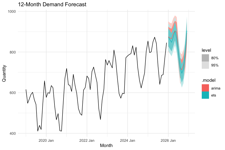
This runs in under a minute on a standard laptop and produces forecasts with prediction intervals that directly inform safety stock calculations. The 80% interval tells your planner: "demand will fall within this range four out of five months." That is a fundamentally more useful input to inventory planning than a single-point estimate in a spreadsheet.

Apply this to your top 50 material groups by spend, and you have a demand planning system that outperforms most manual forecasting processes.

Where to Start

Pick one capability from this list — demand forecasting is usually the easiest win — and apply it to a single material group or product family. Use data you already have in your ERP system. R and Python are free, and the code examples above run on a standard laptop.

The goal is not to build a data science department. It is to answer one operational question better than your current process does, prove the value, and expand from there.