$2,700 Per Year — On a Single Component
Maria manages procurement at a mid-size electronics distributor. Last quarter, her CFO asked a simple question: "Why do we order Component X 50 times a year?" Maria didn’t have a good answer. She’d been ordering 200 units at a time for two years because "it’s about what we need."
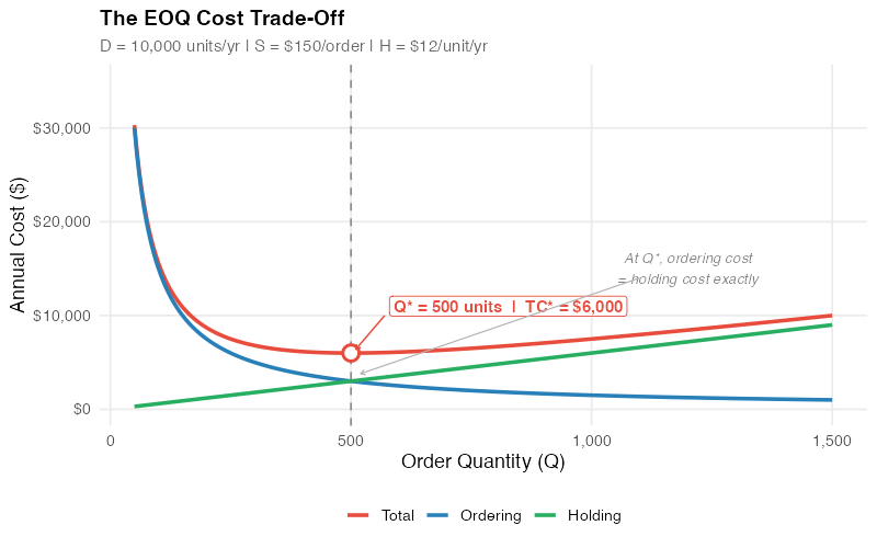
So she ran the numbers. Her company uses 10,000 units of Component X per year. Each order costs $150 to process — purchase order, receiving, quality inspection, accounts payable. Holding a unit in inventory for a year costs $12 in warehousing, insurance, capital, and obsolescence risk. At 200 units per order, she places 50 orders a year.
The math says she should be ordering 500 units at a time — 20 orders instead of 50. Her current approach costs $8,700 per year in ordering and holding costs. The optimal: $6,000. That’s $2,700 per year wasted on a single component. Across the 2,000 SKUs she manages, the gap runs into hundreds of thousands of dollars.
The formula that would have caught this? It was published in 1913 by Ford W. Harris, a former engineer at Westinghouse Electric. It predates sliced bread (1928) and electronic computers by decades. It fits on a Post-it note. And despite a century of advances in computing, AI, and supply chain technology, some variant of it still determines order quantities at the majority of companies worldwide.
The formula is the Economic Order Quantity (EOQ):
Q = sqrt(2DS / H)*
Where D is annual demand, S is the cost per order, and H is the holding cost per unit per year. Three inputs, one square root, done. For Maria’s Component X:
Q = sqrt(2 x 10,000 x $150 / $12) = sqrt(250,000) = 500 units*
The intuition: ordering too frequently wastes money on processing costs. Ordering too much at once wastes money on holding costs. EOQ finds the exact point where these two forces balance — and as we’ll see, the balance point is remarkably forgiving of errors.
The Math: Where Ordering Cost Meets Holding Cost
The total relevant cost (excluding the purchase price, which doesn’t change with order quantity in the basic model) is:
TC(Q) = (D / Q) x S + (Q / 2) x H
The first term is annual ordering cost: you place D/Q orders per year, each costing S. The second term is annual holding cost: your average inventory is Q/2 (you receive Q units and draw them down to zero before reordering), and each unit costs H per year to hold.
Taking the derivative and setting it to zero gives us Q*. But the really beautiful thing happens when you plug Q* back into the cost equation:
At Q, ordering cost = holding cost exactly.*
| Metric | Maria’s Current (Q = 200) | EOQ (Q* = 500) |
|---|---|---|
| Orders per year | 50 | 20 |
| Annual ordering cost | $7,500 | $3,000 |
| Average inventory | 100 units | 250 units |
| Annual holding cost | $1,200 | $3,000 |
| Total relevant cost | $8,700 | $6,000 |
| Cost vs. optimal | +45% | Optimal |
Maria is ordering too frequently. Her ordering cost ($7,500) dwarfs her holding cost ($1,200) — a clear sign that Q is too small. At EOQ, the two costs are perfectly balanced at $3,000 each, and the total drops by $2,700.
The Surprising Robustness: Why a 100-Year-Old Formula Still Works
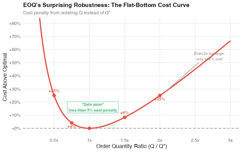
Here’s the part that most textbooks mention in a footnote but should be the headline: EOQ is extraordinarily forgiving.
The cost penalty for using the wrong Q follows this elegant formula:
TC(Q) / TC(Q) = 0.5 x (Q/Q + Q/Q*)**
This function has a remarkably flat bottom. The practical implications are stunning:
| Q / Q* Ratio | You Ordered… | Cost Penalty |
|---|---|---|
| 0.50 | 50% too few | +25% |
| 0.75 | 25% too few | +4.2% |
| 1.00 | Exactly right | 0% |
| 1.25 | 25% too many | +2.5% |
| 1.50 | 50% too many | +8.3% |
| 2.00 | 100% too many | +25% |
Even if you’re off by 50% — ordering 250 or 750 instead of 500 — your cost is only 8-25% above optimal. Get within 25% of Q* and you’re paying less than 5% extra. This is why EOQ survives in practice: the cost curve has a wide, flat valley around the optimum, and being approximately right is almost as good as being exactly right.
This robustness also explains why "round number" ordering works surprisingly well. If Q* = 487 and you order 500 because it’s a nice round number, you’re paying less than 0.04% extra. Round up to fill a pallet? You’re fine. The formula gives you the target; reality gives you the constraint; and the flat bottom means the compromise costs almost nothing.
What If Your Parameters Are Wrong?
The robustness story gets even better. In the real world, you don’t know D and H precisely. Demand fluctuates. Holding costs are estimates. How badly does EOQ perform when your inputs are wrong?
The answer: not badly at all. If your demand estimate is off by 30% and your holding cost estimate is off by 30% in opposite directions (the worst case), your cost penalty is still only about 5%. If the errors happen to go in the same direction (both overestimated or both underestimated), they partially cancel out, and the penalty is even smaller.
This is a mathematical consequence of the square root in the formula. EOQ takes the square root of (2DS/H), so a 30% error in D becomes roughly a 14% error in Q*. The formula dampens your mistakes.
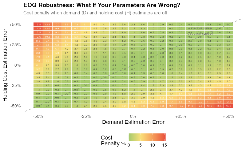
The heatmap shows cost penalties for various combinations of estimation errors. The green zone — where the penalty is under 2% — covers a surprisingly large area. The message is clear: you don’t need perfect data to get near-perfect results from EOQ.
This is the real reason the formula has survived for over a century. Not because supply chains are simple (they aren’t), and not because the assumptions are realistic (they aren’t). It survives because it is robust — the output is remarkably insensitive to errors in the input.
Where EOQ Breaks: Five Failure Modes
So if EOQ is this robust, why does anyone get ordering wrong? Because robustness to parameter errors doesn’t mean robustness to assumption violations. The formula assumes constant demand, fixed prices, unlimited storage, and independent items. Violate those assumptions, and the flat-bottom safety net disappears.
Here are five situations where the basic formula gives misleading answers — and what to do instead.
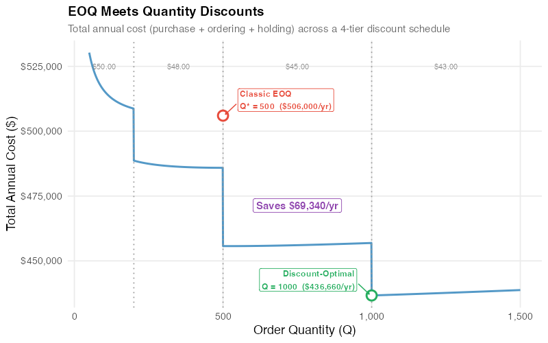
1. Quantity Discounts
The classic EOQ formula assumes a fixed unit price regardless of order size. In reality, suppliers offer lower prices for larger orders. This creates a fundamentally different optimization problem: should you order more than Q* to capture a price break?
The answer is often yes — and the analysis is not trivial. As we explored in detail in the Quantity Discount Analysis post, all-units discount schedules create a sawtooth-shaped total cost curve with discontinuities at each tier boundary. The "roller-coaster effect" means that a lower quoted price doesn’t always mean a lower incremental cost.
The algorithm for EOQ with quantity discounts:
- Compute Q* for each price tier (since H often depends on unit price)
- If Q* falls within the tier’s quantity range, it’s feasible — compute TC at that Q
- If Q* falls below the tier’s minimum, evaluate TC at the tier’s minimum quantity
- Pick the Q with the lowest total annual cost (purchase + ordering + holding)
2. Capacity Constraints
EOQ assumes you can order and store any quantity. In practice, warehouses have finite space, trucks have weight limits, and suppliers have production capacity. If Q* exceeds your storage capacity, you can’t use it.
The fix is constrained optimization: minimize TC subject to Q <= capacity. The constrained optimum is simply min(Q*, capacity) — but this needs to be checked, not assumed.
3. Perishable and Obsolescent Items
EOQ’s holding cost H is typically modeled as a carrying charge (capital cost + storage + insurance). For perishable goods — food, pharmaceuticals, seasonal fashion — there’s an additional cost: expiry. If units expire before they’re sold, the holding cost effectively becomes infinite beyond a certain shelf life.
For fashion or technology products with short life cycles, the obsolescence risk makes large orders dangerous. Ordering 500 units of a component that might be superseded in 3 months is not the same as ordering 500 units of a commodity fastener.
4. Correlated Multi-Item Ordering
EOQ treats each SKU independently. But if you order 50 items from the same supplier, placing 50 separate orders doesn’t make sense — you’d consolidate them into one shipment to share the fixed ordering cost.
Joint replenishment policies coordinate orders across items. The math gets more complex (NP-hard in the general case), but simple heuristics like "power-of-two" policies — where each item’s reorder interval is a power of two times some base period — get within 6% of optimal.
5. Variable Demand
The "D" in EOQ is assumed constant. Real demand isn’t. When demand has significant variability (coefficient of variation above 15-20%), the deterministic EOQ fails to account for the risk of stockouts between orders.
The solution is the (Q, R) policy: keep the EOQ for the order quantity Q, but add a statistically calculated reorder point R that includes safety stock:
R = d x L + z x sigma x sqrt(L)
Where d is average demand per period, L is lead time, z is the service level z-score, and sigma is demand standard deviation. This hybrid approach captures the best of both worlds: EOQ’s cost optimization for the "how much" question, plus statistical rigor for the "when to reorder" question.
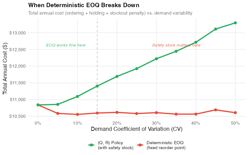
The chart shows the cost divergence: when demand variability is low (CV < 15%), deterministic EOQ works fine. As variability rises, the (Q, R) policy with proper safety stock increasingly outperforms — because it avoids the expensive stockouts that naive EOQ ignores.
The Real-World Cost of Ignoring EOQ
In 2004, researchers Quintana and Nabors published a case study of a U.S. Air Force depot that had been using experience-based ordering for decades. When they applied EOQ analysis to 30 high-volume parts, they found average order quantities were 40% above optimal, generating over $200,000 in excess annual holding costs — at a single facility. The fix required no new software, no new hires, just a spreadsheet and the formula.
That result generalizes. A mid-size distributor handling 5,000 SKUs with an average annual demand of $2 million in inventory can typically expect:
- Gut-feel ordering (typical state): average 30-40% above optimal TC, translating to $150,000–$200,000 per year in excess ordering and holding costs.
- Basic EOQ implementation: gets within 5-10% of optimal, saving $100,000–$150,000 per year.
- EOQ + quantity discount optimization: adds another 3-5% savings on purchase cost — potentially $60,000–$100,000 on a $2M spend.
- Full (Q, R) with safety stock optimization: reduces stockout costs by 40-60% while cutting safety stock by 15-25%.
The return on investment for implementing EOQ-based ordering is almost always measured in weeks, not months. The formula is free. The data — demand, ordering cost, holding cost — is already in your ERP system. The only barrier is organizational inertia.
Interactive Dashboard
Explore the data yourself — plug in your own demand, costs, and discount schedules to see how EOQ optimizes your ordering decisions in real time.
Interactive Dashboard
Explore the data yourself — adjust parameters and see the results update in real time.
Your Next Steps
-
Pull your top 20 SKUs by spend and compute Q for each.* The formula is Q* = sqrt(2DS/H). Use annual demand from your ERP, estimate ordering cost at $50-$200 per order (include everyone’s time: purchasing, receiving, inspection, AP), and holding cost at 20-30% of unit value per year. Compare Q* to your current order quantities. The R code below automates this.
-
Check for the "Maria problem." If your ordering cost far exceeds your holding cost (or vice versa), you’re not at Q*. The two should be roughly equal. A 3:1 ratio means you’re ordering too frequently (or too infrequently), and rebalancing will save real money.
-
Run your supplier quotes through Quantity Discount Analysis (QDA). For any SKU where you’re offered quantity discounts, the basic EOQ isn’t enough. Use the quantity discount algorithm to find the true optimal Q. The interactive dashboard and R code handle this automatically.
-
Add safety stock where CV > 15%. For items with significant demand variability, upgrade from pure EOQ to (Q, R). The formula R = dL + zsigma*sqrt(L) with z = 1.645 (95% service level) is a practical starting point. The simulation in the R code shows exactly when this matters.
-
Benchmark and iterate. Compute your current total relevant cost, implement EOQ-based ordering for your top SKUs, and measure the before-and-after difference. Most organizations see payback within the first ordering cycle.
Show R Code
# =============================================================================
# EOQ Analysis and Optimization
# =============================================================================
# A complete R toolkit for Economic Order Quantity analysis, sensitivity
# testing, quantity discount optimization, and variable demand simulation.
#
# Required packages: ggplot2, dplyr, tidyr, scales, patchwork
# =============================================================================

library(ggplot2)
library(dplyr)
library(tidyr)
library(scales)
library(patchwork)

# --- Theme for all plots ---
theme_eoq <- theme_minimal(base_size = 13) +
  theme(
    plot.title = element_text(face = "bold", size = 14),
    plot.subtitle = element_text(color = "grey40", size = 11),
    panel.grid.minor = element_blank(),
    legend.position = "bottom"
  )

# =============================================================================
# 1. CORE EOQ FUNCTIONS
# =============================================================================

# Classic EOQ formula
eoq <- function(D, S, H) {
  sqrt(2 * D * S / H)
}

# Total relevant cost (ordering + holding, excludes purchase)
tc_relevant <- function(Q, D, S, H) {
  (D / Q) * S + (Q / 2) * H
}

# Total cost including purchase
tc_total <- function(Q, D, S, H, P) {
  D * P + (D / Q) * S + (Q / 2) * H
}

# Cost penalty ratio: TC(Q) / TC(Q*)
cost_penalty <- function(Q, Q_star) {
  0.5 * (Q_star / Q + Q / Q_star)
}

# =============================================================================
# 2. EXAMPLE PARAMETERS
# =============================================================================

D <- 10000   # Annual demand (units)
S <- 150     # Ordering cost per order ($)
H <- 12      # Holding cost per unit per year ($)
P <- 50      # Unit price ($)

Q_star <- eoq(D, S, H)
TC_star <- tc_relevant(Q_star, D, S, H)

cat(sprintf("EOQ (Q*) = %.0f units\n", Q_star))
cat(sprintf("Optimal orders/year = %.0f\n", D / Q_star))
cat(sprintf("Optimal TC (ordering + holding) = $%s\n", comma(round(TC_star))))
cat(sprintf("Ordering cost at Q* = $%s\n", comma(round((D / Q_star) * S))))
cat(sprintf("Holding cost at Q*  = $%s\n", comma(round((Q_star / 2) * H))))

# =============================================================================
# 3. CHART 1 — Total Cost Curves
# =============================================================================

Q_range <- seq(50, 1500, by = 5)

cost_df <- data.frame(Q = Q_range) %>%
  mutate(
    Ordering = (D / Q) * S,
    Holding  = (Q / 2) * H,
    Total    = Ordering + Holding
  )

cost_long <- cost_df %>%
  pivot_longer(cols = c(Ordering, Holding, Total),
               names_to = "Component", values_to = "Cost") %>%
  mutate(Component = factor(Component,
    levels = c("Total", "Ordering", "Holding")))

p1 <- ggplot(cost_long, aes(x = Q, y = Cost, color = Component, linetype = Component)) +
  geom_line(linewidth = 1.2) +
  geom_vline(xintercept = Q_star, linetype = "dashed", color = "grey40", alpha = 0.7) +
  geom_point(data = data.frame(Q = Q_star, Cost = TC_star,
             Component = factor("Total", levels = c("Total", "Ordering", "Holding"))),
             aes(x = Q, y = Cost), size = 4, shape = 21, fill = "white",
             stroke = 1.5, color = "#e74c3c") +
  annotate("text", x = Q_star + 30, y = TC_star + 800,
           label = paste0("Q* = ", round(Q_star), " units\nTC* = $", comma(round(TC_star))),
           hjust = 0, size = 3.8, color = "#e74c3c", fontface = "bold") +
  annotate("text", x = Q_star + 30, y = TC_star / 2 - 200,
           label = "At Q*, ordering cost\n= holding cost exactly",
           hjust = 0, size = 3.2, color = "grey50", fontface = "italic") +
  scale_color_manual(values = c("Total" = "#e74c3c", "Ordering" = "#2980b9",
                                 "Holding" = "#27ae60")) +
  scale_linetype_manual(values = c("Total" = "solid", "Ordering" = "solid",
                                    "Holding" = "solid")) +
  scale_x_continuous(labels = comma_format()) +
  scale_y_continuous(labels = dollar_format(), limits = c(0, 35000)) +
  labs(
    title = "The EOQ Cost Trade-Off",
    subtitle = sprintf("D = %s units/yr | S = $%s/order | H = $%s/unit/yr",
                       comma(D), comma(S), H),
    x = "Order Quantity (Q)",
    y = "Annual Cost ($)",
    color = NULL, linetype = NULL
  ) +
  theme_eoq

ggsave("https://inphronesys.com/wp-content/uploads/2026/02/eoq_cost_curves-4.png", p1,
       width = 8, height = 5, dpi = 100, bg = "white")

# =============================================================================
# 4. CHART 2 — Sensitivity / Cost Penalty Curve
# =============================================================================

ratio_range <- seq(0.2, 3.0, by = 0.01)

sensitivity_df <- data.frame(ratio = ratio_range) %>%
  mutate(
    cost_penalty = 0.5 * (1 / ratio + ratio),
    pct_above = (cost_penalty - 1) * 100
  )

key_points <- data.frame(
  ratio = c(0.5, 0.75, 1.0, 1.5, 2.0),
  label = c("50% too small", "25% too small", "Optimal Q*",
            "50% too large", "100% too large")
) %>%
  mutate(
    cost_penalty = 0.5 * (1 / ratio + ratio),
    pct_above = (cost_penalty - 1) * 100
  )

p2 <- ggplot(sensitivity_df, aes(x = ratio, y = pct_above)) +
  geom_line(linewidth = 1.3, color = "#e74c3c") +
  geom_hline(yintercept = 0, linetype = "dashed", color = "grey50") +
  geom_ribbon(data = sensitivity_df %>% filter(ratio >= 0.6, ratio <= 1.7),
              aes(ymin = 0, ymax = pct_above),
              fill = "#27ae60", alpha = 0.1) +
  annotate("text", x = 1.15, y = 3,
           label = "\"Safe zone\"\n< 5% cost penalty",
           color = "#27ae60", size = 3.5, fontface = "bold") +
  geom_point(data = key_points, aes(x = ratio, y = pct_above),
             size = 3, color = "#e74c3c") +
  geom_text(data = key_points %>% filter(ratio != 1.0),
            aes(x = ratio, y = pct_above, label = sprintf("+%.0f%%", pct_above)),
            vjust = -1.2, size = 3.5, fontface = "bold", color = "#e74c3c") +
  annotate("text", x = 2.5, y = 40,
           label = "Even 2x too large:\nonly +25% cost",
           color = "grey40", size = 3.2, fontface = "italic") +
  annotate("segment", x = 2.3, xend = 2.05, y = 38, yend = 27,
           arrow = arrow(length = unit(0.15, "cm")), color = "grey60") +
  scale_x_continuous(breaks = seq(0.5, 3.0, by = 0.5),
                     labels = function(x) paste0(x, "x")) +
  scale_y_continuous(breaks = seq(0, 80, by = 10),
                     labels = function(x) paste0("+", x, "%")) +
  coord_cartesian(ylim = c(-2, 80)) +
  labs(
    title = "EOQ's Surprising Robustness: The Flat-Bottom Cost Curve",
    subtitle = "Cost penalty from ordering Q instead of Q*",
    x = "Order Quantity Ratio (Q / Q*)",
    y = "Cost Increase Above Optimal"
  ) +
  theme_eoq

ggsave("https://inphronesys.com/wp-content/uploads/2026/02/eoq_sensitivity-4.png", p2,
       width = 8, height = 5, dpi = 100, bg = "white")

# =============================================================================
# 5. CHART 3 — Robustness Heatmap
# =============================================================================

errors <- seq(-0.50, 0.50, by = 0.05)

heatmap_df <- expand.grid(D_err = errors, H_err = errors) %>%
  mutate(
    D_true = D * (1 + D_err),
    H_true = H * (1 + H_err),
    Q_used = sqrt(2 * D * S / H),
    Q_true = sqrt(2 * D_true * S / H_true),
    TC_yours = (D_true / Q_used) * S + (Q_used / 2) * H_true,
    TC_true  = (D_true / Q_true) * S + (Q_true / 2) * H_true,
    penalty_pct = (TC_yours / TC_true - 1) * 100
  )

p3 <- ggplot(heatmap_df, aes(x = D_err * 100, y = H_err * 100, fill = penalty_pct)) +
  geom_tile(color = "white", linewidth = 0.3) +
  geom_text(aes(label = sprintf("%.1f", penalty_pct)),
            size = 2.2, color = ifelse(heatmap_df$penalty_pct > 5, "white", "grey20")) +
  geom_abline(slope = 1, intercept = 0, linetype = "dashed",
              color = "grey40", alpha = 0.5) +
  annotate("text", x = 35, y = 42,
           label = "Errors in same\ndirection cancel",
           color = "grey40", size = 3, fontface = "italic") +
  scale_fill_gradient2(
    low = "#27ae60", mid = "#f9e07a", high = "#e74c3c",
    midpoint = 5, name = "Cost\nPenalty %"
  ) +
  scale_x_continuous(breaks = seq(-50, 50, by = 25),
                     labels = function(x) paste0(ifelse(x > 0, "+", ""), x, "%")) +
  scale_y_continuous(breaks = seq(-50, 50, by = 25),
                     labels = function(x) paste0(ifelse(x > 0, "+", ""), x, "%")) +
  labs(
    title = "EOQ Robustness: What If Your Parameters Are Wrong?",
    subtitle = "Cost penalty when demand (D) and holding cost (H) estimates are off",
    x = "Demand Estimation Error",
    y = "Holding Cost Estimation Error"
  ) +
  theme_eoq +
  theme(panel.grid = element_blank())

ggsave("https://inphronesys.com/wp-content/uploads/2026/02/eoq_robustness_heatmap-4.png", p3,
       width = 8, height = 5, dpi = 100, bg = "white")

# =============================================================================
# 6. CHART 4 — EOQ vs Quantity Discount
# =============================================================================

discounts <- data.frame(
  tier = 1:4,
  qty_min = c(1, 200, 500, 1000),
  qty_max = c(199, 499, 999, 2000),
  price   = c(50.00, 48.00, 45.00, 43.00)
)

Q_disc_range <- 50:1500

tc_discount <- data.frame(Q = Q_disc_range) %>%
  rowwise() %>%
  mutate(
    tier_idx = max(which(discounts$qty_min <= Q)),
    unit_price = discounts$price[tier_idx],
    TC_total = D * unit_price + (D / Q) * S + (Q / 2) * (unit_price * 0.24)
  ) %>%
  ungroup()

eoq_per_tier <- discounts %>%
  mutate(
    H_tier = price * 0.24,
    Q_eoq  = sqrt(2 * D * S / H_tier),
    Q_feasible = pmax(qty_min, pmin(qty_max, Q_eoq)),
    TC_at_feasible = D * price + (D / Q_feasible) * S + (Q_feasible / 2) * H_tier
  )

Q_classic <- sqrt(2 * D * S / H)
TC_classic <- D * P + (D / Q_classic) * S + (Q_classic / 2) * H
best_tier <- eoq_per_tier %>% slice_min(TC_at_feasible, n = 1)

p4 <- ggplot(tc_discount, aes(x = Q, y = TC_total)) +
  geom_line(linewidth = 1, color = "#2980b9", alpha = 0.8) +
  geom_vline(xintercept = c(200, 500, 1000), linetype = "dotted", color = "grey60") +
  annotate("text", x = 100, y = max(tc_discount$TC_total) * 0.98,
           label = "Tier 1\n$50.00", color = "grey50", size = 2.8) +
  annotate("text", x = 350, y = max(tc_discount$TC_total) * 0.98,
           label = "Tier 2\n$48.00", color = "grey50", size = 2.8) +
  annotate("text", x = 750, y = max(tc_discount$TC_total) * 0.98,
           label = "Tier 3\n$45.00", color = "grey50", size = 2.8) +
  annotate("text", x = 1250, y = max(tc_discount$TC_total) * 0.98,
           label = "Tier 4\n$43.00", color = "grey50", size = 2.8) +
  geom_point(data = data.frame(Q = round(Q_classic),
             TC_total = TC_classic),
             size = 4, shape = 21, fill = "white", stroke = 1.5, color = "#e74c3c") +
  annotate("text", x = Q_classic + 30, y = TC_classic + 3000,
           label = paste0("Classic EOQ\nQ* = ", round(Q_classic),
                          "\nTC = $", comma(round(TC_classic))),
           hjust = 0, size = 3.2, color = "#e74c3c", fontface = "bold") +
  geom_point(data = data.frame(Q = best_tier$Q_feasible,
             TC_total = best_tier$TC_at_feasible),
             size = 4, shape = 21, fill = "white", stroke = 1.5, color = "#27ae60") +
  annotate("text", x = best_tier$Q_feasible + 30,
           y = best_tier$TC_at_feasible - 3000,
           label = paste0("Discount-Optimal\nQ = ", round(best_tier$Q_feasible),
                          "\nTC = $", comma(round(best_tier$TC_at_feasible))),
           hjust = 0, size = 3.2, color = "#27ae60", fontface = "bold") +
  scale_x_continuous(labels = comma_format()) +
  scale_y_continuous(labels = dollar_format()) +
  labs(
    title = "EOQ Meets Quantity Discounts",
    subtitle = "Total annual cost across a 4-tier discount schedule",
    x = "Order Quantity (Q)",
    y = "Total Annual Cost ($)"
  ) +
  theme_eoq

ggsave("https://inphronesys.com/wp-content/uploads/2026/02/eoq_vs_discount-4.png", p4,
       width = 8, height = 5, dpi = 100, bg = "white")

# =============================================================================
# 7. CHART 5 — EOQ vs (Q,R) Under Variable Demand
# =============================================================================

set.seed(42)

simulate_eoq_vs_qr <- function(D_annual, S, H, cv, n_weeks = 1000) {
  D_weekly <- D_annual / 52
  sigma_weekly <- D_weekly * cv

  demands <- pmax(0, rnorm(n_weeks, mean = D_weekly, sd = sigma_weekly))

  # Policy 1: Deterministic EOQ with fixed reorder point
  Q_eoq <- sqrt(2 * D_annual * S / H)
  R_eoq <- D_weekly * 2

  inv_eoq <- numeric(n_weeks)
  inv_eoq[1] <- Q_eoq + R_eoq
  orders_eoq <- 0
  stockouts_eoq <- 0

  for (t in 2:n_weeks) {
    inv_eoq[t] <- inv_eoq[t - 1] - demands[t]
    if (inv_eoq[t] < R_eoq) {
      inv_eoq[t] <- inv_eoq[t] + Q_eoq
      orders_eoq <- orders_eoq + 1
    }
    if (inv_eoq[t] < 0) {
      stockouts_eoq <- stockouts_eoq + abs(inv_eoq[t])
      inv_eoq[t] <- 0
    }
  }

  # Policy 2: (Q, R) with safety stock
  L <- 2
  sigma_L <- sigma_weekly * sqrt(L)
  z <- 1.645
  R_qr <- D_weekly * L + z * sigma_L
  Q_qr <- sqrt(2 * D_annual * S / H)

  inv_qr <- numeric(n_weeks)
  inv_qr[1] <- Q_qr + R_qr
  orders_qr <- 0
  stockouts_qr <- 0

  for (t in 2:n_weeks) {
    inv_qr[t] <- inv_qr[t - 1] - demands[t]
    if (inv_qr[t] < R_qr) {
      inv_qr[t] <- inv_qr[t] + Q_qr
      orders_qr <- orders_qr + 1
    }
    if (inv_qr[t] < 0) {
      stockouts_qr <- stockouts_qr + abs(inv_qr[t])
      inv_qr[t] <- 0
    }
  }

  years <- n_weeks / 52

  tc_eoq <- (orders_eoq / years) * S +
    mean(pmax(inv_eoq, 0)) * H +
    (stockouts_eoq / years) * 50

  tc_qr <- (orders_qr / years) * S +
    mean(pmax(inv_qr, 0)) * H +
    (stockouts_qr / years) * 50

  data.frame(
    cv = cv,
    EOQ_TC = tc_eoq,
    QR_TC  = tc_qr,
    EOQ_SL = 1 - stockouts_eoq / sum(demands),
    QR_SL  = 1 - stockouts_qr / sum(demands)
  )
}

cv_values <- seq(0, 0.50, by = 0.05)
variability_results <- bind_rows(lapply(cv_values, function(cv) {
  simulate_eoq_vs_qr(D, S, H, cv)
}))

cat("\n=== EOQ vs (Q,R) Under Variable Demand ===\n")
print(variability_results %>%
  mutate(across(c(EOQ_TC, QR_TC), ~dollar(round(.)))) %>%
  mutate(across(c(EOQ_SL, QR_SL), ~percent(., accuracy = 0.1))))

# =============================================================================
# 8. EOQ WITH QUANTITY DISCOUNTS — Algorithm
# =============================================================================

eoq_with_discounts <- function(D, S, discount_schedule, holding_pct = 0.24) {
  # Evaluates EOQ across all tiers and finds the global optimum.
  #
  # Args:
  #   D: annual demand
  #   S: ordering cost per order
  #   discount_schedule: data frame with tier, qty_min, qty_max, price
  #   holding_pct: holding cost as percentage of unit price
  #
  # Returns: data frame with feasible Q and TC for each tier, plus the winner

  results <- discount_schedule %>%
    mutate(
      H_tier = price * holding_pct,
      Q_eoq  = sqrt(2 * D * S / H_tier),
      # Feasibility: Q must be within the tier's range
      Q_feasible = case_when(
        Q_eoq >= qty_min & Q_eoq <= qty_max ~ Q_eoq,  # within range
        Q_eoq < qty_min ~ qty_min,                      # bump up to tier min
        TRUE ~ NA_real_                                  # Q exceeds tier max; skip
      ),
      TC = ifelse(!is.na(Q_feasible),
                  D * price + (D / Q_feasible) * S + (Q_feasible / 2) * H_tier,
                  NA_real_),
      is_optimal = FALSE
    ) %>%
    filter(!is.na(TC))

  # Mark the winner
  results$is_optimal[which.min(results$TC)] <- TRUE
  results
}

cat("\n=== EOQ with Quantity Discounts ===\n")
result <- eoq_with_discounts(D, S, discounts)
print(result %>% select(tier, qty_min, qty_max, price, Q_eoq, Q_feasible, TC, is_optimal))

# =============================================================================
# 9. APPLY TO YOUR OWN DATA
# =============================================================================
#
# To run EOQ analysis on your own SKUs:
#
# 1. Create a data frame with your SKU parameters:
#
#    my_skus <- data.frame(
#      sku    = c("COMP-001", "COMP-002", "COMP-003"),
#      D      = c(5000, 12000, 800),     # annual demand
#      S      = c(120, 120, 120),         # ordering cost (often the same)
#      H      = c(8.50, 15.00, 3.20),     # holding cost per unit per year
#      P      = c(42.50, 75.00, 16.00),   # unit price
#      Q_curr = c(200, 500, 100)          # current order quantity
#    )
#
# 2. Compute EOQ and savings:
#
#    my_skus <- my_skus %>%
#      mutate(
#        Q_star     = sqrt(2 * D * S / H),
#        TC_current = (D / Q_curr) * S + (Q_curr / 2) * H,
#        TC_optimal = sqrt(2 * D * S * H),
#        savings    = TC_current - TC_optimal,
#        pct_over   = (TC_current / TC_optimal - 1) * 100
#      )
#
#    print(my_skus)
#    cat(sprintf("Total annual savings: $%s\n", comma(round(sum(my_skus$savings)))))
#
# 3. For SKUs with quantity discounts, use:
#
#    my_discounts <- data.frame(
#      tier    = 1:3,
#      qty_min = c(1, 100, 500),
#      qty_max = c(99, 499, 2000),
#      price   = c(42.50, 40.00, 37.50)
#    )
#    eoq_with_discounts(D = 5000, S = 120, my_discounts)
References
- Harris, F.W. (1913). "How Many Parts to Make at Once." Factory, The Magazine of Management, 10(2), 135-136, 152. (The original EOQ paper — yes, from 1913.)
- Wilson, R.H. (1934). "A Scientific Routine for Stock Control." Harvard Business Review, 13(1), 116-128. (Popularized Harris’s formula; sometimes called the Wilson formula.)
- Erlenkotter, D. (1990). "Ford Whitman Harris and the Economic Order Quantity Model." Operations Research, 38(6), 937-946. (The definitive history of EOQ’s origins.)
- Zipkin, P.H. (2000). Foundations of Inventory Management. McGraw-Hill. (Comprehensive treatment of EOQ extensions and stochastic models.)
- Axsater, S. (2015). Inventory Control. Springer. (Modern treatment including (Q, R) policies and multi-echelon systems.)
Schreibe einen Kommentar