Every time series tells three stories at once.
There’s the long arc — the trend. Is demand growing? Shrinking? Flattening out? Then there’s the rhythm — the seasonality. Summer peaks, winter troughs, end-of-quarter spikes from customers gaming their own budgets. And finally, there’s everything else — the remainder, the noise, the “what on earth happened in March 2024?” part that no pattern can explain.
The problem is that when you look at a raw time series, you hear all three stories simultaneously. It’s like listening to a symphony with the melody, harmony, and percussion layered on top of each other — beautiful to experience, impossible to analyze. You can’t tune the violins if you can’t isolate them from the cellos.
Last week, we learned to see our data — eight chart types that reveal hidden patterns in demand data. We popped the hood. Today, we take the engine apart.
Time series decomposition is the statistical technique that separates a time series into its component parts: trend, seasonality, and remainder. It’s one of the most powerful diagnostic tools in the forecaster’s toolkit, and it’s been evolving for over a century — from the crude methods of the 1920s to sophisticated algorithms that can handle multiple seasonal patterns, holidays, and abrupt structural changes.
By the end of this post, you’ll understand not just how decomposition works, but which method to use for your specific data. That distinction matters more than most textbooks let on.
The Three Components (And Why They Matter for Planning)
Mathematically, decomposition models a time series y_t as a combination of three components:
- Trend-cycle (T_t): The long-term direction and medium-term cycles. In supply chain terms, this is your underlying demand trajectory — market growth, product lifecycle, gradual customer base changes.
- Seasonal (S_t): Repeating patterns with a fixed, known period. Quarterly budget cycles, summer demand peaks, December retail surges, Monday warehouse volume spikes. The key word is fixed — if the pattern repeats at the same interval, it’s seasonal.
- Remainder (R_t): Everything that isn’t trend or seasonality. Promotions, supply disruptions, one-time events, random variation. The “unexplained” part — and often the most interesting part to investigate.
The question is: how do these three components combine?
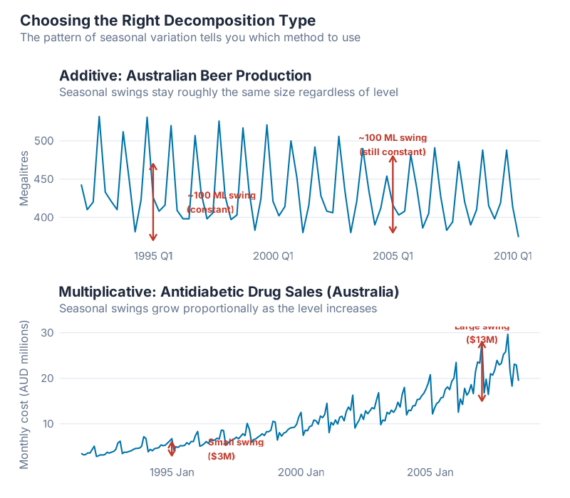
Additive vs. Multiplicative: The Decision That Shapes Everything
In an additive model, the components simply add up:
y_t = S_t + T_t + R_t
This means seasonal swings are roughly constant in absolute terms. If your product sells 200 extra units every December regardless of whether baseline demand is 1,000 or 5,000, that’s additive seasonality.
In a multiplicative model, the components multiply:
y_t = S_t x T_t x R_t
Here, seasonal swings scale proportionally with the level. If December demand is always about 20% higher than baseline — whether baseline is 1,000 (so +200) or 5,000 (so +1,000) — that’s multiplicative seasonality.
Why this matters for your supply chain: Get this choice wrong and your seasonal factors will be systematically biased. Additive factors applied to multiplicative data will underestimate peaks at high demand levels and overestimate them at low levels. Your safety stock calculations, production plans, and procurement schedules all inherit that error.
The practical test: Plot your data. If the seasonal “amplitude” (the distance from peak to trough) stays roughly constant as the level changes, use additive. If it grows proportionally with the level, use multiplicative. When in doubt, there’s an elegant trick: apply a log transformation to your data. Since log(S_t x T_t x R_t) = log(S_t) + log(T_t) + log(R_t), taking logarithms converts a multiplicative model into an additive one. Decompose the log-transformed series additively, then exponentiate back. Problem solved.
Most retail and consumer goods demand data is multiplicative — higher-volume products have proportionally larger seasonal swings. Most industrial and MRO data is closer to additive. But always check. Your data doesn’t care about rules of thumb.
Moving Averages: The Foundation of Trend Estimation
Before we decompose anything, we need a way to estimate the trend. The classic tool is the moving average — and despite its simplicity, it’s worth understanding properly, because every decomposition method builds on this idea.
An m-order moving average estimates the trend at time t by averaging m consecutive observations centered around t:
T̂t = (1/m) (y{t-(m-1)/2} + … + y_t + … + y_{t+(m-1)/2})
For odd values of m, this is straightforward — a 5-MA averages the two observations before, the current one, and the two after. For even periods (like monthly data with m = 12), you need a small adjustment: the 2xm-MA, which takes a moving average of the moving average to re-center it. A 2×12-MA is the standard approach for monthly data.
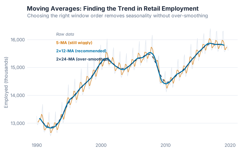
What you’re seeing: Lower-order moving averages (m = 3, m = 5) follow the data closely but don’t fully remove the seasonal pattern. Higher-order averages (m = 12 for monthly data) smooth out the seasonality entirely, revealing the pure trend underneath. The 2×12-MA is the sweet spot for monthly supply chain data — it removes the 12-month seasonal cycle while preserving the trend.
There’s a trade-off here that mirrors a fundamental tension in supply chain planning: responsiveness vs. stability. A short moving average responds quickly to changes but is noisy. A long moving average is stable but slow to react. Sound familiar? It’s the same trade-off you face choosing between responsive and stable safety stock parameters, or between short and long planning horizons in your MRP.
Weighted moving averages generalize this by assigning different weights to each observation (weights must sum to 1 and be symmetric). The 2×12-MA is actually a weighted MA where the first and last observations get half weight. This matters because it means the trend estimate is less influenced by extreme values at the edges of the window.
Classical Decomposition: Where It All Started
Classical decomposition has been around since the 1920s — longer than most supply chain concepts. It’s beautifully simple, which is both its charm and its fatal flaw.
The Algorithm (Additive Version)
- Estimate the trend using a 2xm-MA (e.g., 2×12-MA for monthly data)
- Detrend the data by subtracting the trend: y_t – T̂_t
- Estimate the seasonal component by averaging the detrended values for each season (all Januaries together, all Februaries together, etc.), then adjusting so the seasonal factors sum to zero over a complete cycle
- Calculate the remainder: R_t = y_t – T̂_t – Ŝ_t
For the multiplicative version, replace subtraction with division in steps 2 and 4.
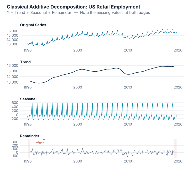
What you’re seeing: The top panel is the original series. Below it, the smooth trend-cycle estimated by the 2×12-MA. Then the seasonal component — a repeating pattern that’s identical every year (this is a critical limitation we’ll discuss). And finally the remainder, which should ideally look like random noise if the decomposition captured everything meaningful.
Why Hyndman Says “Not Recommended”
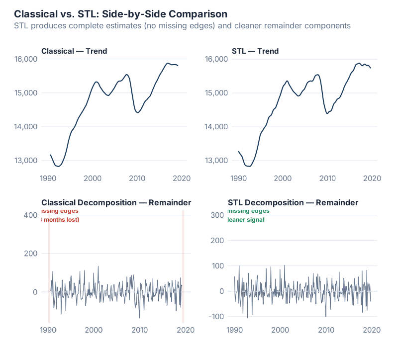
Classical decomposition is still taught — and still used in many supply chain organizations — but Rob Hyndman’s verdict in Forecasting: Principles and Practice is blunt: “not recommended.” Here’s why:
- Missing edges. The 2xm-MA can’t produce estimates for the first and last m/2 observations. For a 2×12-MA on monthly data, you lose the first 6 and last 6 months. That’s a full year of your most recent data — exactly the part you care about most for planning.
- Over-smoothing. The trend estimate can smooth out rapid changes, like a sudden demand shift from a new product launch or a lost customer. The MA just averages right through it, as if nothing happened.
- Static seasonality. Classical decomposition assumes the seasonal pattern is identical every year. That’s almost never true in practice. Consumer preferences shift. Product mixes change. Supply chains reconfigure. A method that can’t handle evolving seasonality is going to drift further from reality every year.
- Outlier sensitivity. A single unusual observation — a massive one-time order, a data entry error, a pandemic — gets absorbed into the seasonal and trend estimates, contaminating both. There’s no mechanism to say “that point is weird, let’s downweight it.”
These aren’t minor quibbles. They’re structural problems that make classical decomposition unreliable for real forecasting work. It’s like using a typewriter in 2026 — historically interesting, good for understanding the concept, but you wouldn’t build your production plan on it.
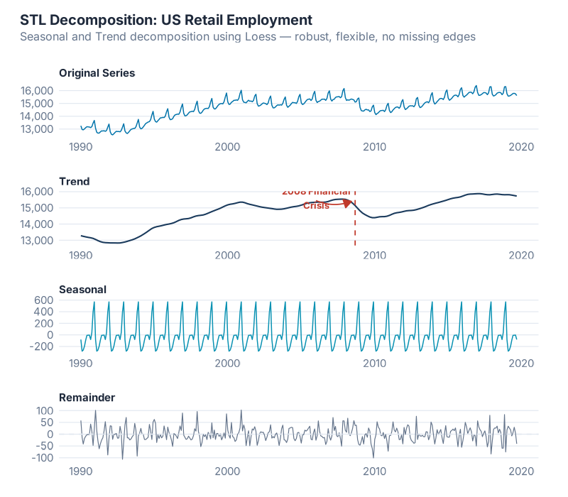
STL: The Method You Should Actually Be Using
STL — Seasonal and Trend decomposition using LOESS — was developed by Cleveland, Cleveland, McRae, and Terpenning in 1990, and it remains the workhorse of modern time series decomposition. If classical decomposition is the typewriter, STL is the word processor.
How STL Works
Instead of simple moving averages, STL uses LOESS (LOcally Estimated Scatterplot Smoothing) — a form of local weighted regression that fits smooth curves through data points by giving more weight to nearby observations. The algorithm alternates between two nested loops:
Inner loop (runs multiple times per iteration):
- Remove the current seasonal estimate from the data
- Apply LOESS smoothing to estimate the trend
- Remove the trend estimate from the data
- Apply LOESS smoothing to estimate the seasonality
- Repeat until convergence
Outer loop (for robustness):
- Calculates weights based on the size of each remainder value
- Large remainders (potential outliers) get downweighted
- The inner loop re-runs with these weights, so outliers have less influence
This iterative LOESS-based approach is what gives STL its superpowers:
Why STL Beats Classical (Every Time)
| Feature | Classical | STL |
|---|---|---|
| Handles any seasonal period | Limited | Yes — daily, weekly, monthly, any |
| Evolving seasonality | No — static pattern | Yes — seasonal shape can change over time |
| Adjustable smoothness | No — fixed | Yes — tune trend and seasonal windows |
| Robust to outliers | No | Yes — via outer loop weighting |
| Edge estimates | Missing first/last m/2 | Available for the full series |
Evolving seasonality is the game-changer. In the real world, your December peak might be getting stronger every year as e-commerce grows. Your Q3 trough might be shifting as your customer base changes regions. STL captures this because it re-estimates the seasonal component at every time point, rather than averaging all Decembers together and assuming they’re identical.
The Two Parameters That Matter
STL has several parameters, but two dominate:
season(window = ...)— Controls how quickly the seasonal component can change. Larger values mean more stable seasonality (closer to classical decomposition). Smaller values allow the seasonal pattern to evolve more freely. A common starting point for monthly data isseason(window = 13), which uses just over one year’s worth of data to estimate each seasonal value.trend(window = ...)— Controls how smooth the trend is. Larger values produce smoother trends. Smaller values let the trend respond to shorter-term changes. A rough rule of thumb: set it to about 1.5 times the seasonal period, then adjust based on what the remainder looks like.
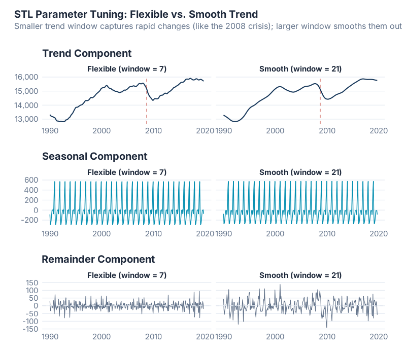
What you’re seeing: The same data decomposed with three different parameter settings. Narrow windows (left) produce a wiggly trend and rapidly changing seasonality — responsive but noisy. Wide windows (right) produce a smooth trend and near-constant seasonality — stable but potentially missing real changes. The middle ground is where the art meets the science.
The diagnostic trick: Look at the remainder. If it shows obvious patterns — clear seasonality, systematic trends — your decomposition hasn’t captured everything. Go back and adjust. A good decomposition produces a remainder that looks like white noise (random, unpatterned, centered on zero).
STL’s Limitations
STL isn’t perfect. Two limitations matter for supply chain work:
- Additive only. STL natively handles additive decomposition. For multiplicative data, you need to log-transform first, decompose, then exponentiate back. It works, but it’s an extra step and the back-transformed confidence intervals can be asymmetric.
- No calendar adjustment. STL treats every month (or quarter, or week) as equally long. It doesn’t know that February has fewer days than March, or that some months have five Mondays while others have four. For daily-level supply chain data — warehouse throughput, order volumes — this can matter.
The Payoff: Seasonally Adjusted Data
One of the most valuable outputs of decomposition isn’t a forecast — it’s the seasonally adjusted series. By removing the seasonal component, you can see the underlying trend and unusual events without the seasonal noise:
Seasonally adjusted = y_t – Ŝ_t (additive)
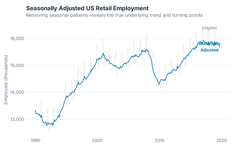
Why supply chain teams should care: Seasonally adjusted data makes it much easier to detect real changes in underlying demand. Did that jump in March represent genuine demand growth, or was it just the seasonal March peak? Subtracting out the seasonal component gives you the answer. It’s also what central banks and government statisticians use when they report “seasonally adjusted” GDP or employment figures — the same technique, applied at a very different scale.
Beyond STL: Modern Decomposition Methods
STL was published in 1990. A lot has happened in 36 years. The core idea — iterative LOESS smoothing — remains sound, but researchers have extended it to handle increasingly complex real-world data. Here are three methods pushing the frontier.
MSTL: Multiple Seasonal Patterns
MSTL (Multiple Seasonal-Trend decomposition using LOESS), developed by Bandara, Hyndman, and Bergmeir, extends STL to handle data with multiple seasonal patterns simultaneously.
Why does this matter? Because much real-world supply chain data has more than one seasonal cycle. Daily warehouse data might have both a weekly pattern (lower volumes on weekends) and an annual pattern (holiday peaks in December). Hourly electricity demand has daily cycles (morning ramp-up, evening peak), weekly cycles (weekday vs. weekend), and annual cycles (summer cooling, winter heating).
STL can only handle one seasonal period at a time. You could nest multiple STL passes, but the order of decomposition affects the results, and parameter tuning becomes a nightmare. MSTL handles all seasonal patterns in a single, principled algorithm — and with fewer tuning parameters than alternatives like Prophet or TBATS.
In fpp3, you can use MSTL directly with the STL() function by specifying multiple seasonal periods. It’s already built into the tidyverts ecosystem.
STAHL: When Holidays Break Your Patterns
STAHL (Seasonal, Trend, and Holiday Decomposition with LOESS) is a 2025 innovation from Quantcube Technology that adds something STL and MSTL can’t handle: an explicit holiday component.
Think about it: Easter moves. Chinese New Year moves. Ramadan moves. These events create demand spikes (or dips) that don’t align with fixed seasonal periods. STL dumps them into the remainder. Your seasonal factors end up contaminated by holiday effects that shift from year to year, and your remainder contains systematic patterns that aren’t truly random.
STAHL solves this with three key innovations:
- Spectral frequency identification — automatically detects which seasonal periods are present in the data, rather than requiring you to specify them
- Explicit holiday component — separates holiday effects from the regular seasonal pattern
- Second inner loop — disentangles outliers from holiday effects (a distinction that earlier methods blur together)
The results are striking: in automated quality assessments, STAHL showed a 42% improvement over comparable methods on key decomposition quality metrics. For supply chain data with significant holiday effects — retail, food & beverage, consumer electronics — this is a major advance.
BASTION: Bayesian Decomposition with Uncertainty
BASTION (Bayesian Adaptive Seasonality and Trend DecompositION) takes a fundamentally different approach. Instead of LOESS smoothing, it uses a Bayesian framework to decompose time series into trend and multiple seasonal components.
What makes BASTION interesting for supply chain applications:
- Uncertainty quantification: Every component estimate comes with a credible interval. You don’t just get “the trend is going up” — you get “the trend is going up, and we’re 95% confident it’s between X and Y.” For safety stock calculations and scenario planning, this is gold.
- Abrupt change handling: BASTION can detect and adapt to sudden level shifts — a new customer, a lost contract, a supply chain disruption that permanently alters your demand pattern. STL’s LOESS smoothing tends to gradually absorb these shifts rather than detecting them cleanly.
- Robustness to outliers: The Bayesian framework naturally handles unusual observations through its probabilistic model, without needing a separate robustness loop.
BASTION is still relatively new and not yet part of the standard fpp3 toolkit, but it represents where the field is heading: probabilistic decomposition that quantifies what we know and what we don’t.
X-11 and SEATS: The Official Statistics Workhorses
No discussion of decomposition is complete without mentioning the methods used by statistical agencies worldwide. X-11 (developed at the U.S. Census Bureau) and SEATS (developed at the Bank of Spain) are the backbone of official economic statistics — the methods behind every “seasonally adjusted employment figure” and “seasonally adjusted GDP growth rate” you’ve ever seen in the news.
The modern implementation, X-13ARIMA-SEATS, combines both approaches with ARIMA modeling for trend extension. In R, the seasonal package by Christoph Sax provides a clean interface:
library(seasonal)
seas_model <- seas(AirPassengers)
plot(seas_model)
For most supply chain applications, STL or MSTL will serve you better — X-11/SEATS are optimized for the specific needs of macroeconomic statistics (calendar adjustment, trading day effects, holiday correction) that matter less for demand planning. But if your organization needs to produce official or regulatory-grade seasonally adjusted figures, these are the methods to use.
Method Comparison: Choosing the Right Tool
Here’s the cheat sheet. Every method has trade-offs — there is no single “best” decomposition method for all data.
| Criterion | Classical | STL | X-11 / SEATS | MSTL | STAHL | BASTION |
|---|---|---|---|---|---|---|
| Evolving seasonality | No | Yes | Yes | Yes | Yes | Yes |
| Multiple seasonal periods | No | No | No | Yes | Yes | Yes |
| Robust to outliers | No | Yes | Partial | Yes | Yes | Yes |
| Holiday handling | No | No | Yes (X-11) | No | Yes | No |
| Uncertainty estimates | No | No | No | No | No | Yes |
| Calendar adjustment | No | No | Yes | No | Yes | No |
| Ease of use in R | Easy | Easy (fpp3) | Moderate (seasonal) |
Easy (fpp3) | Specialized | Specialized |
| Best for | Teaching | General use | Official statistics | Complex seasonality | Holiday-heavy data | Scenario planning |
The decision tree for supply chain forecasters:
- Single seasonal period, no holidays? Use STL. It’s the default for good reason.
- Multiple seasonal periods (e.g., daily data with weekly + annual cycles)? Use MSTL.
- Significant holiday effects (retail, consumer goods)? Consider STAHL or X-11.
- Need uncertainty bands on components for planning? Watch BASTION as it matures.
- Government reporting or official statistics? Use X-13ARIMA-SEATS via the
seasonalpackage. - Just learning? Start with STL. Seriously. It handles 90% of cases well, and everything else is a refinement.
Interactive Dashboard
Explore the decomposition methods yourself — adjust parameters, switch between additive and multiplicative models, and see how different STL window settings change the results in real time.
Interactive Dashboard
Explore the data yourself — adjust parameters and see the results update in real time.
Your Next Steps
Decomposition is a diagnostic tool, not a forecast. It tells you what’s inside your time series so you can make better modeling decisions. Here are five things you can do with this knowledge right now:
- Decompose one real demand series this week. Pick your highest-volume SKU, pull 3+ years of monthly data, and run
STL()in fpp3. Look at the remainder — does it look random? If not, your current forecast model is missing something. - Check your additive/multiplicative assumption. Plot your data. If seasonal amplitude grows with the level, log-transform before decomposing. Getting this wrong silently biases every seasonal factor downstream.
- Use seasonally adjusted data in your next S&OP meeting. When someone says “demand jumped 15% last month,” pull out the seasonally adjusted series and check — was it a real jump, or just the seasonal March peak? You’ll be the smartest person in the room.
- Compare your ERP’s seasonal factors to STL’s. Many ERP systems use classical decomposition (or worse, static seasonal indices that haven’t been updated in years). Run STL on the same data and compare. The differences will tell you how much forecast accuracy you’re leaving on the table.
- Read ahead. Next week, we’ll use what we’ve learned here — the trend, the seasonality, the choice between additive and multiplicative — to build actual forecast models with ETS and ARIMA. Decomposition was the diagnosis. Forecasting is the treatment.
Show R Code
# =============================================================================
# Time Series Decomposition in R — Complete Reproducible Code
# =============================================================================
# This code accompanies the blog post on inphronesys.com
# All examples use the fpp3 ecosystem (tidyverts)
# =============================================================================

# --- Load packages ---
library(fpp3)        # Loads tsibble, tsibbledata, feasts, fable, ggplot2, etc.
library(patchwork)   # Multi-panel plot layouts
library(slider)      # Efficient moving average calculations
library(scales)      # Axis label formatting

source("Scripts/theme_inphronesys.R")

# --- Prepare the data ---
# US Retail Employment (monthly, 1990 onward)
retail <- us_employment |>
  filter(year(Month) >= 1990, Title == "Retail Trade") |>
  select(Month, Employed)

# =============================================================================
# Step 1: Understand Additive vs. Multiplicative Decomposition
# =============================================================================

# Additive: Y = Trend + Seasonal + Remainder
#   Use when seasonal swings stay CONSTANT regardless of level
beer <- aus_production |>
  filter(year(Quarter) >= 1992) |>
  select(Quarter, Beer)

autoplot(beer, Beer) +
  labs(title = "Beer Production — Constant Seasonal Amplitude (Additive)")

# Multiplicative: Y = Trend × Seasonal × Remainder
#   Use when seasonal swings GROW with the level
a10 <- PBS |>
  filter(ATC2 == "A10") |>
  summarise(Cost = sum(Cost))

autoplot(a10, Cost) +
  labs(title = "Drug Sales — Growing Seasonal Amplitude (Multiplicative)")

# =============================================================================
# Step 2: Moving Averages — Estimating the Trend
# =============================================================================

retail_ma <- retail |>
  as_tibble() |>
  mutate(
    MA_5    = slide_dbl(Employed, mean, .before = 2, .after = 2, .complete = TRUE),
    ma12    = slide_dbl(Employed, mean, .before = 5, .after = 6, .complete = TRUE),
    MA_2x12 = slide_dbl(ma12, mean, .before = 0, .after = 1, .complete = TRUE)
  )

# =============================================================================
# Step 3: Classical Decomposition
# =============================================================================

retail |>
  model(classical_decomposition(Employed, type = "additive")) |>
  components() |>
  autoplot() +
  labs(title = "Classical Additive Decomposition")

# =============================================================================
# Step 4: STL Decomposition (the modern standard)
# =============================================================================

dcmp <- retail |>
  model(STL(Employed ~ trend(window = 13) + season(window = "periodic"))) |>
  components()

autoplot(dcmp) +
  labs(title = "STL Decomposition of US Retail Employment")

# =============================================================================
# Step 5: Tuning STL Parameters
# =============================================================================

# Compare flexible vs. smooth trend windows
stl_flex <- retail |>
  model(STL(Employed ~ trend(window = 7) + season(window = "periodic"))) |>
  components()

stl_smooth <- retail |>
  model(STL(Employed ~ trend(window = 21) + season(window = "periodic"))) |>
  components()

# =============================================================================
# Step 6: Extracting the Seasonally Adjusted Series
# =============================================================================

dcmp |>
  as_tibble() |>
  mutate(
    Month = as.Date(Month),
    Seasonally_Adjusted = Employed - season_year
  ) |>
  ggplot(aes(x = Month)) +
  geom_line(aes(y = Employed), color = "grey80") +
  geom_line(aes(y = Seasonally_Adjusted), color = "#0073aa") +
  labs(
    title = "Original vs. Seasonally Adjusted",
    y = "Employed (thousands)", x = NULL
  )

# =============================================================================
# Step 7: Comparing Methods
# =============================================================================

# Ljung-Box test for autocorrelation in remainder:
dcmp |>
  as_tsibble() |>
  features(remainder, ljung_box, lag = 24)

# =============================================================================
# Apply to Your Own Data
# =============================================================================

# Replace this with your own time series:
#
# my_data <- read_csv("your_data.csv") |>
#   mutate(Date = yearmonth(Date)) |>
#   as_tsibble(index = Date)
#
# # Visualize first
# autoplot(my_data, Value)
#
# # Check: additive or multiplicative?
# # If seasonal swings grow → use log transform for additive
# my_data <- my_data |> mutate(Log_Value = log(Value))
#
# # Decompose with STL
# my_dcmp <- my_data |>
#   model(STL(Value ~ trend(window = 13) + season(window = "periodic"))) |>
#   components()
#
# # Inspect components
# autoplot(my_dcmp)
#
# # Extract seasonally adjusted series
# my_sa <- my_dcmp |>
#   as_tibble() |>
#   mutate(SA = Value - season_year)
References
- Hyndman, R.J., & Athanasopoulos, G. (2021). Forecasting: Principles and Practice, 3rd edition. OTexts. Chapter 3: Time Series Decomposition. otexts.com/fpp3/decomposition.html
- Cleveland, R.B., Cleveland, W.S., McRae, J.E., & Terpenning, I. (1990). STL: A Seasonal-Trend Decomposition Procedure Based on Loess (with Discussion). Journal of Official Statistics, 6(1), 3–73.
- Bandara, K., Hyndman, R.J., & Bergmeir, C. (2025). MSTL: A Seasonal-Trend Decomposition Algorithm for Time Series with Multiple Seasonal Patterns. International Journal of Operational Research, 52(1), 79–98.
- Haller, V., Daniel, S., & Bellone, B. (2025). STAHL: Seasonal, Trend, and Holiday Decomposition with Loess. Journal of Official Statistics, 41(4).
- Sax, C., & Eddelbuettel, D. (2018). Seasonal Adjustment by X-13ARIMA-SEATS in R. Journal of Statistical Software, 87(11), 1–17.
- Persons, W.M. (1919). Indices of Business Conditions. Review of Economics and Statistics, 1, 5–107. (Early classical decomposition methods.)
Leave a Reply