Four datasets. Same mean. Same variance. Same correlation. Same regression line.

Completely different shapes.

This is Anscombe’s Quartet — a famous statistical demonstration from 1973, and the single best argument for why you should plot your data before you do anything else with it. All four datasets produce identical summary statistics: mean of X = 9, mean of Y ≈ 7.5, variance nearly identical, and a correlation coefficient of r ≈ 0.816 across all four. Your ERP’s summary dashboard would show you the same numbers for each one and tell you everything is fine.

Now look at what happens when you actually plot them:

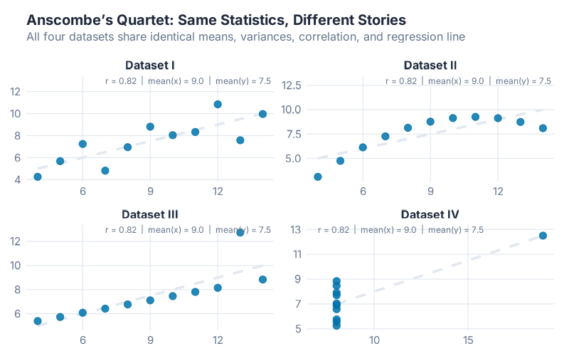
Dataset I is the only one that fits a linear model. Dataset II is a perfect curve — the linear model is completely wrong. Dataset III has a single outlier dragging the line off course. And Dataset IV? The entire correlation is driven by one extreme point. Remove it and the relationship disappears.

Same numbers. Four completely different stories. And if you hadn’t plotted them, you’d have treated all four identically — with a straight line and a confident MAPE.

This is what happens in supply chain forecasting every single day. Someone pulls 36 months of demand data, calculates an average growth rate, fits a trend, and sends the forecast to the S&OP meeting. Nobody plots it. Nobody checks whether the pattern is linear, curved, seasonal, or driven by a single outlier month when a customer accidentally ordered 10x their normal quantity and then returned half of it.

"The first thing to do in any data analysis task is to plot the data. Graphs enable many features of the data to be visualised, including patterns, unusual observations, changes over time, and relationships between variables." — Hyndman & Athanasopoulos, Forecasting: Principles and Practice

Hyndman is right. And today, I’m going to show you the visual toolkit that makes plotting supply chain data not just easy, but genuinely fun. By the end of this post, you’ll have eight chart types in your arsenal — five from fpp3 and three bonus ones that go beyond the textbook — and you’ll never look at a demand summary table the same way again.

Your Line Chart Is Lying to You

In our first post this month, we showed why R crushes Excel for forecasting. Last time, you installed R, RStudio, and fpp3, and produced your first real forecast. But we skipped a step. A critical one.

We went straight from data to model. We didn’t look at the data first.

That’s like a mechanic replacing your engine without popping the hood. Sure, a new engine might fix the problem. But what if the issue was a loose spark plug?

Every forecasting model makes assumptions about your data. ETS assumes a certain error structure. ARIMA assumes stationarity (or that differencing achieves it). Even Seasonal Naive assumes the seasonal pattern is stable. If those assumptions are wrong — if your data has a structural break, or an outlier, or a changing seasonal pattern — the model will happily fit itself to garbage and give you a confident-looking garbage forecast.

Visualization is how you check those assumptions before you bet your inventory on them. And fpp3 gives you a visual toolkit specifically designed for time series data — not just generic scatter plots, but purpose-built charts that each reveal a different hidden pattern.

Let’s meet the toolkit. We’ll use Australian quarterly beer production as our primary dataset for the core fpp3 charts — so you can see how each visualization reveals something new about data you’ve already "seen." Then we’ll explore three creative techniques with different data to show their unique strengths.

The fpp3 Visual Toolkit

1. autoplot() — The Time Plot

The most basic visualization, and the one most teams skip. autoplot() plots your time series as a line chart with proper time axis formatting. Two lines of code:

beer <- aus_production |>
  filter(year(Quarter) >= 1992) |>
  select(Quarter, Beer)

beer |> autoplot(Beer)

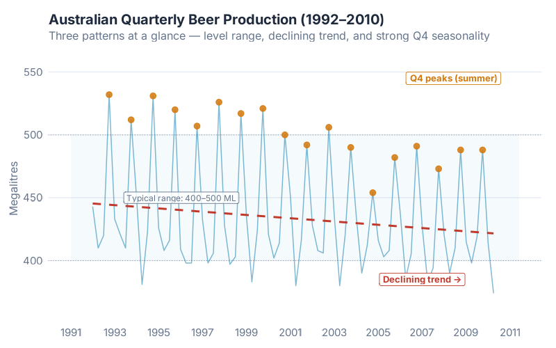
What this tells a supply chain pro: You immediately see three things — the overall level (roughly 400–500 megalitres per quarter), a slight downward trend over time, and a strong seasonal pattern that repeats every year. That seasonal pattern is Q4-dominant — Australians drink more beer in their summer (October–December). You also see that the variability is roughly constant — the seasonal swings don’t get bigger or smaller, which tells you additive seasonality is probably appropriate.

This is the chart you should have run before that S&OP meeting. It takes ten seconds and saves you from building a forecast on data you haven’t actually looked at.

2. gg_season() — The Seasonal Overlay

Now we go deeper. gg_season() takes each year of data and overlays them on top of each other, all sharing the same x-axis (Q1 through Q4). This lets you compare the seasonal shape across years instantly:

beer |> gg_season(Beer, labels = "both")

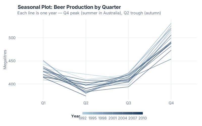
What this tells a supply chain pro: Is the seasonal pattern stable? Getting stronger? Shifting? This chart answers all three at a glance. You can see that Q4 is consistently the peak and Q2 is consistently the trough — but the peak has been getting slightly lower over the years. The overall "shape" of the season is stable, but the level is declining. If your seasonal factors in Excel haven’t been updated since 2005, this chart tells you they need revision.

This is how you discover that your December spike has been creeping into November for three years. Or that your Q3 pre-build has shifted from August to July. Or that one year’s pattern was completely anomalous — and your model is treating it as normal.

Your ERP vendor charges six figures for a dashboard that can’t do gg_season().

3. gg_subseries() — The Subseries Means

This one is less well known, and it’s a gem. gg_subseries() splits your data into mini-panels — one per season (quarter, in our case). Within each panel, you see the observations for that quarter over time. And the horizontal blue line shows the mean for that period:

beer |> gg_subseries(Beer)

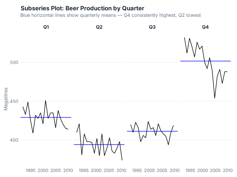
What this tells a supply chain pro: Is each season trending the same way, or are some quarters changing while others hold steady? Look at Q4 — it’s clearly declining. But Q2 might be more stable. That distinction matters enormously for planning: if your peak season is eroding while your trough stays flat, your overall demand is contracting, and your seasonal factors need to shrink the peak amplitude.

This is the chart that tells you Q4 production has been declining for 15 years. And makes you ask: did anyone notice? Was this deliberate (market shift, health trends, category decline) or did it slip under the radar while everyone focused on the annual total?

4. gg_lag() — The Lag Scatter Plot

This chart asks: does last quarter’s production predict this quarter’s production? And if so, which lags matter most?

beer |> gg_lag(Beer, lags = 1:9)

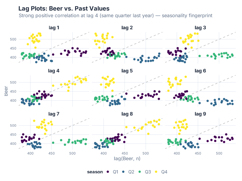
What this tells a supply chain pro: Each panel plots the current quarter’s value (y-axis) against the value k quarters ago (x-axis). If you see a tight cluster along the diagonal, that lag is a strong predictor. The color coding shows which quarter each point belongs to.

Look at lag 4 — that’s the "same quarter last year" comparison. If that panel shows a tight linear relationship, it means last year’s Q4 is a good predictor of this year’s Q4. That’s Seasonal Naive in visual form. If lag 1 also shows a tight relationship, recent momentum matters too. If only lag 4 is tight and lag 1 is scattered, your data is seasonal but not autoregressive — a critical distinction for model selection.

This is the chart that tells you whether "last quarter predicts this quarter" or "same quarter last year predicts this quarter." Your model choice depends on the answer. And yes, we just diagnosed a model selection problem by looking at a scatter plot of beer production. Sometimes the best tools are the simplest — and the ones that pair well with an actual beer.

5. ACF Plot — The Autocorrelation Fingerprint

The ACF (AutoCorrelation Function) plot is the single most information-dense chart in time series analysis. It summarizes the correlation structure of your entire dataset in one compact graph:

beer |> ACF(Beer) |> autoplot()

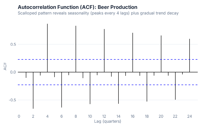
What this tells a supply chain pro: Read it like a diagnostic scan. Three patterns to look for:

• Slowly decaying bars = your data has a trend. The current value is correlated with many past values because they’re all riding the same trend.
• Spikes at seasonal lags (4, 8, 12 for quarterly data) = your data has seasonality. Values are correlated with the same season in previous years.
• Scalloped pattern (decay + spikes) = your data has both trend and seasonality. This is the most common pattern in supply chain data.

The blue dashed lines mark the significance threshold. Bars that extend beyond them represent statistically significant autocorrelation. For beer data, you’ll see the scalloped pattern — confirmation that this data has both trend and seasonal components, which tells you an ETS or seasonal ARIMA model is appropriate.

Three seconds of looking at this chart and you know whether ETS or ARIMA is the better starting point. Three seconds. Compare that to the hours people spend "tuning" models without first understanding their data’s correlation structure.

Beyond the Textbook

The five fpp3 charts above cover the essentials. But there are visualization techniques that go beyond what the textbook teaches — charts that are visually striking, immediately intuitive, and perfect for presentations where you need to make a point in under five seconds.

6. Ridgeline Plot — Distribution Mountains

A ridgeline plot (sometimes called a joy plot) stacks yearly distributions like mountain ranges, showing how the shape of your data changes over time. It uses the ggridges package (install it once with install.packages("ggridges")):

library(ggridges)
beer |>
  mutate(Year = factor(year(Quarter))) |>
  ggplot(aes(x = Beer, y = Year)) +
  geom_density_ridges()

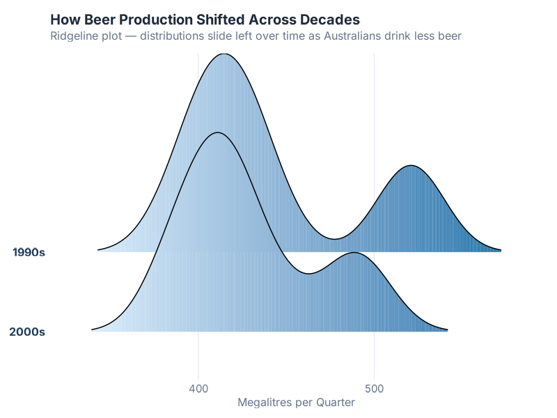
What this tells a supply chain pro: If your demand volatility is increasing, a ridgeline plot screams it at you. Wider "mountains" = more spread in that year’s values. If the mountains are getting wider over time, your demand is becoming harder to predict. If they’re shifting left or right, your baseline level is changing. And if one year has a weird double-peak shape, something structural happened that year.

This chart is a showstopper in presentations. Your warehouse manager will stop scrolling. Your VP will ask "what’s that?" And you’ll say "that’s our demand volatility by year, and it’s getting worse." Good luck getting that reaction from a pivot table.

7. Calendar Heatmap — The GitHub Contribution Graph

You’ve seen GitHub’s green contribution squares? Same idea, but for your warehouse data. Each cell represents a single day, arranged in a weekday × week grid, colored by order volume. Daily data is where this chart shines — it reveals patterns that weekly or monthly aggregation hides completely:

orders |>
  mutate(
    week = isoweek(date),
    weekday = wday(date, label = TRUE)
  ) |>
  ggplot(aes(x = week, y = weekday, fill = volume)) +
  geom_tile()

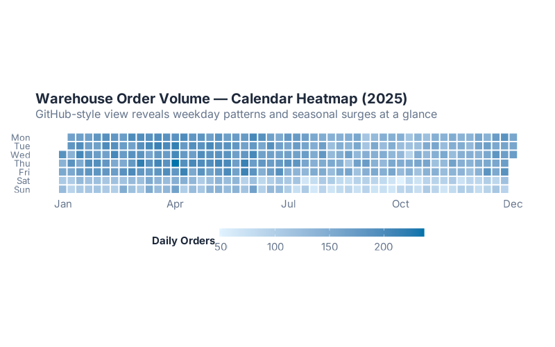
What this tells a supply chain pro: Patterns jump off the screen. Monday order spikes from the weekend backlog. Friday dips because nobody submits purchase orders at 4 PM on a Friday. A dead week in August when the factory was shut down for maintenance. That one Wednesday in March that’s inexplicably hot — turns out a customer placed their entire quarter’s worth of orders in a single day.

Your warehouse manager will understand this chart in two seconds. No statistics degree required. No explanation of autocorrelation needed. Dark square = high demand. Pattern of dark squares = recurring pattern. Done.

8. Month × Year Tile Heatmap — Ten Years in One Image

The tile heatmap puts months on the y-axis, years on the x-axis, and encodes the value as color. It’s the most compact way to show both seasonality AND trend simultaneously:

a10_data |>
  ggplot(aes(x = year, y = month, fill = cost)) +
  geom_tile() +
  scale_fill_viridis_c()

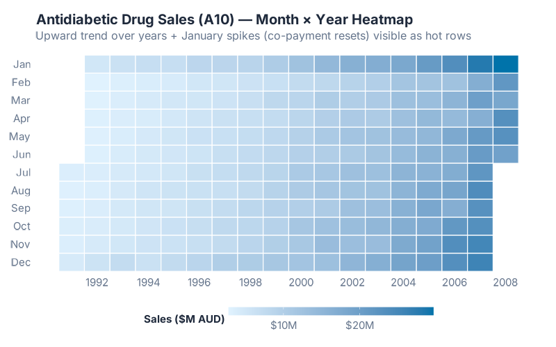
What this tells a supply chain pro: Read it two ways. Read across a row: you see the trend for that month over years. Read down a column: you see the seasonal pattern for that year. Read the overall gradient from top-left to bottom-right: you see the combined trend and seasonality at once. Fifteen years of monthly data in a single image.

For the a10 antidiabetic drug data, the heatmap reveals something autoplot hints at but doesn’t make obvious — January is consistently the hottest month. Why? Australia’s Pharmaceutical Benefits Scheme resets its safety net threshold on January 1, so patients rush to fill extra prescriptions in late December while subsidies still apply — but those sales aren’t registered until January due to government reporting lags. That spike has nothing to do with disease epidemiology — it’s a government policy artifact. And the overall trend is unmistakable: the colors get hotter from left to right as costs increase year over year.

This chart is devastating in S&OP meetings. Instead of flipping through twelve monthly charts or squinting at a line plot with 180 data points, you show one image and say "here’s everything." The trend is obvious, the seasonality is obvious, and anomalies pop out as cells that don’t match their neighbors.

The 30-Second Rule

Here’s my challenge to you. Before your next forecast — before you open your model, before you tune parameters, before you touch a single smoothing constant — spend 30 seconds plotting the data three different ways:

1. autoplot() — see the big picture
2. gg_season() — check if the seasonal pattern is stable
3. ACF — read the autocorrelation fingerprint

If what you see surprises you, your forecast was about to be wrong.

A trend you didn’t know about. A seasonal shift that started two years ago. An outlier from that month when the warehouse flooded and everything got backordered. These are the things that break forecasts — and they’re invisible in summary tables but obvious in the right chart.

The fpp3 toolkit gives you these charts in one or two lines of code each. No formatting. No wrestling with Excel chart axes. No "why did the legend move when I resized the window." Just data in, insight out.

And if you want to go further — ridgeline plots, heatmaps, calendar grids — R’s visualization ecosystem is effectively unlimited. The charts in this post are the starting lineup. The bench goes deep.

Interactive Dashboard

Explore the visual toolkit yourself — switch between chart types, change datasets, and discover patterns in real time.

What’s Next

Today we learned to see our data. Next time, we learn to decompose it — breaking a time series into its trend, seasonal, and remainder components to understand the structure hiding underneath the noise. If today was "pop the hood and look," next time is "take the engine apart and understand every piece."

Because once you can see the trend, the seasonality, and the noise separately, choosing the right forecasting model stops being a guessing game. It becomes obvious.

See you next time.

# =============================================================================
# Time Series Graphics with fpp3 — Full Reproducible Code
# =============================================================================
# Generates all visualizations from this blog post
# Install once: install.packages(c("fpp3", "ggridges"))

source("Scripts/theme_inphronesys.R")
library(fpp3)
library(ggridges)

# --- Anscombe's Quartet ---------------------------------------------------
# Demonstrates why summary statistics alone are not enough
data(anscombe)

anscombe_long <- tibble(
  x = c(anscombe$x1, anscombe$x2, anscombe$x3, anscombe$x4),
  y = c(anscombe$y1, anscombe$y2, anscombe$y3, anscombe$y4),
  dataset = rep(paste("Dataset", c("I", "II", "III", "IV")), each = 11)
)

ggplot(anscombe_long, aes(x = x, y = y)) +
  geom_point(size = 3, color = iph_colors$blue) +
  geom_smooth(method = "lm", se = FALSE, color = iph_colors$red,
              linewidth = 1) +
  facet_wrap(~dataset, ncol = 2) +
  labs(title = "Anscombe's Quartet",
       subtitle = "All four datasets: mean(x) = 9, mean(y) ≈ 7.5, r ≈ 0.816",
       x = "X", y = "Y") +
  theme_inphronesys()

ggsave("https://inphronesys.com/wp-content/uploads/2026/04/tsgraphics_anscombe-1.png", width = 8, height = 7,
       dpi = 100, bg = "white")

# --- Prepare beer data ----------------------------------------------------
beer <- aus_production |>
  filter(year(Quarter) >= 1992) |>
  select(Quarter, Beer)

# --- 1. autoplot() — Time plot --------------------------------------------
beer |>
  autoplot(Beer) +
  labs(title = "Australian Quarterly Beer Production",
       subtitle = "1992–2010: declining trend with strong Q4 seasonality",
       y = "Megalitres") +
  theme_inphronesys()

ggsave("https://inphronesys.com/wp-content/uploads/2026/04/tsgraphics_autoplot-1.png", width = 8, height = 5,
       dpi = 100, bg = "white")

# --- 2. gg_season() — Seasonal overlay ------------------------------------
beer |>
  gg_season(Beer, labels = "both") +
  labs(title = "Seasonal Plot: Beer Production by Quarter",
       subtitle = "Each colored line is one year — Q4 peak, Q2 trough",
       y = "Megalitres") +
  theme_inphronesys()

ggsave("https://inphronesys.com/wp-content/uploads/2026/04/tsgraphics_season-1.png", width = 8, height = 5,
       dpi = 100, bg = "white")

# --- 3. gg_subseries() — Subseries means ----------------------------------
beer |>
  gg_subseries(Beer) +
  labs(title = "Subseries Plot: Each Quarter's Trend Over Time",
       subtitle = "Blue line = quarter mean — Q4 declining, Q2 stable",
       y = "Megalitres") +
  theme_inphronesys()

ggsave("https://inphronesys.com/wp-content/uploads/2026/04/tsgraphics_subseries-1.png", width = 8, height = 5,
       dpi = 100, bg = "white")

# --- 4. gg_lag() — Lag scatter plots --------------------------------------
beer |>
  gg_lag(Beer, lags = 1:9, geom = "point") +
  labs(title = "Lag Plots: Does Past Production Predict Current?",
       subtitle = "Lag 4 (same quarter last year) shows the tightest relationship") +
  theme_inphronesys()

ggsave("https://inphronesys.com/wp-content/uploads/2026/04/tsgraphics_lag-1.png", width = 8, height = 7,
       dpi = 100, bg = "white")

# --- 5. ACF plot — Autocorrelation fingerprint ----------------------------
beer |>
  ACF(Beer) |>
  autoplot() +
  labs(title = "ACF: The Autocorrelation Fingerprint",
       subtitle = "Scalloped pattern = trend + seasonality") +
  theme_inphronesys()

ggsave("https://inphronesys.com/wp-content/uploads/2026/04/tsgraphics_acf-1.png", width = 8, height = 5,
       dpi = 100, bg = "white")

# --- 6. Ridgeline plot — Distribution mountains ---------------------------
beer |>
  as_tibble() |>
  mutate(Year = factor(year(Quarter))) |>
  ggplot(aes(x = Beer, y = Year, fill = after_stat(x))) +
  geom_density_ridges_gradient(scale = 3, rel_min_height = 0.01) +
  scale_fill_gradient(low = iph_colors$lightgrey, high = iph_colors$blue) +
  labs(title = "Ridgeline Plot: Production Distribution by Year",
       subtitle = "Each ridge shows one year's spread — wider = more variable",
       x = "Megalitres", y = NULL) +
  theme_inphronesys() +
  theme(legend.position = "none")

ggsave("https://inphronesys.com/wp-content/uploads/2026/04/tsgraphics_ridgeline-1.png", width = 8, height = 5,
       dpi = 100, bg = "white")

# --- Prepare a10 antidiabetic drug data -----------------------------------
a10_data <- PBS |>
  filter(ATC2 == "A10") |>
  summarise(Cost = sum(Cost)) |>
  mutate(
    Year  = year(Month),
    Month_name = factor(month(Month, label = TRUE), levels = rev(month.abb))
  ) |>
  as_tibble()

# --- 7. Calendar heatmap (daily warehouse orders) -------------------------
set.seed(42)
dates_daily <- seq(as.Date("2025-01-01"), as.Date("2025-12-31"), by = "day")
weekday_effect <- c(Mon = 1.15, Tue = 1.05, Wed = 1.0, Thu = 0.95,
                    Fri = 0.85, Sat = 0.5, Sun = 0.3)
orders <- tibble(
  date   = dates_daily,
  wday   = wday(dates_daily, label = TRUE),
  week   = isoweek(dates_daily),
  volume = round(150 * weekday_effect[as.character(wday(dates_daily, label = TRUE))] *
                   (1 + 0.2 * sin(2 * pi * yday(dates_daily) / 365)) +
                   rnorm(length(dates_daily), 0, 15))
)

orders |>
  ggplot(aes(x = week, y = fct_rev(wday), fill = volume)) +
  geom_tile(color = "white", linewidth = 0.5) +
  scale_fill_gradient(low = "white", high = iph_colors$blue) +
  labs(title = "Calendar Heatmap: Daily Warehouse Orders (2025)",
       subtitle = "Weekday × week grid — weekday patterns + seasonal variation",
       x = "Week of Year", y = NULL, fill = "Orders") +
  theme_inphronesys() +
  theme(panel.grid = element_blank())

ggsave("https://inphronesys.com/wp-content/uploads/2026/04/tsgraphics_calendar_heatmap-1.png", width = 8, height = 5,
       dpi = 100, bg = "white")

# --- 8. Month × Year tile heatmap ----------------------------------------
a10_data |>
  ggplot(aes(x = Year, y = Month_name, fill = Cost)) +
  geom_tile(color = "white", linewidth = 0.5) +
  scale_fill_viridis_c(option = "inferno", labels = scales::label_comma()) +
  labs(title = "Tile Heatmap: Seasonality × Trend in One View",
       subtitle = "Read across = trend over years | Read down = seasonal pattern",
       x = NULL, y = NULL, fill = "Cost ($M)") +
  theme_inphronesys() +
  theme(panel.grid = element_blank())

ggsave("https://inphronesys.com/wp-content/uploads/2026/04/tsgraphics_tile_heatmap-1.png", width = 8, height = 5,
       dpi = 100, bg = "white")

# =============================================================================
# Try It With Your Own Data
# =============================================================================
# Export your monthly demand from SAP/Oracle/ERP as CSV:
#
# my_data <- read.csv("my_demand.csv") |>
#   mutate(month = yearmonth(date)) |>
#   as_tsibble(index = month)
#
# # The 30-second visual check:
# my_data |> autoplot(demand)           # Big picture
# my_data |> gg_season(demand)          # Seasonal stability
# my_data |> ACF(demand) |> autoplot()  # Autocorrelation fingerprint

References

• Anscombe, F.J. (1973). Graphs in Statistical Analysis. The American Statistician, 27(1), 17-21.
• Hyndman, R.J., & Athanasopoulos, G. (2021). Forecasting: Principles and Practice, 3rd edition, Chapter 2: Time Series Graphics. OTexts. Available free online at otexts.com/fpp3.
• Wilke, C.O. (2019). Fundamentals of Data Visualization. O’Reilly Media.
• Grabowski, J.-P. (2024). R For Purchasing Professionals (RFPP). A practical guide to using R for supply chain data analysis.