In December 2025, researchers at UC San Diego published a peer-reviewed receipt on something the forecasting community has been tiptoeing around for two years: Google’s shiny new time-series foundation model, TimesFM, got beaten by a model older than the first iPhone. By a lot. The winner — vector autoregression (VAR) — has been kicking around since 1980, when Christopher Sims (the eventual 2011 economics Nobel laureate) wrote the paper that made it famous. The score was not close.
At the La Jolla emergency department, forecasting how many patients would be stuck „boarding“ (admitted but not yet in a ward bed), VAR scored an RMSE of 8.76 at the one-day-ahead horizon where it was actually deployed. Google’s TimesFM, at the same T+1 horizon, scored 14.54 — 66% worse than VAR. The 2-week moving average baseline sat at 14.85, which means VAR cut error by 41% versus the naive benchmark — while TimesFM failed to beat that benchmark at any horizon, getting worse as the forecast stretched (RMSE 16.88 at T+4). Out of six candidate models, VAR was the only one the hospital put into live production, quietly emailing forecasts to Mission Control every morning at 7:10.[^1]
If you run a supply chain, that result should stop you mid-coffee. Because the reason VAR won in a hospital is exactly the reason it tends to win in demand planning too — and almost nobody in SCM is using it. This post walks through what VAR actually is (without the matrix algebra), why supply chain data is practically designed for it, and how to build one in R in about thirty lines of code.
What VAR Actually Is
Here’s the one-sentence version: VAR is ARIMA with friends.
An ARIMA model stares intensely at one time series — weekly demand, for example — and tries to predict its next value from its own past. It’s a monk. Deeply introspective. Ignores everything else in the room.
A VAR model, by contrast, watches a small group of related time series at the same time and lets them gossip. Each series predicts its next value using its own past AND the past of every other series in the group. Weekly demand depends on last week’s demand, and on last week’s price, and on last week’s promotion intensity. Price depends on its own past and on demand. Promotions depend on both. Everyone tells on everyone else.
That’s the whole idea. No matrices, no eigenvalues, no doctoral-defence nightmares. Just: if you’ve got three or four series that you suspect talk to each other, VAR lets them actually talk.
The quiet genius of Sims’s 1980 paper „Macroeconomics and Reality“[^2] was philosophical. He argued that economists were imposing too much theoretical structure on their models — deciding in advance that „interest rates cause inflation“ and baking that into the equations. His counter-proposal: let the data decide who causes whom. Treat every variable symmetrically. Regress each one on lagged values of itself and all the others. Read the tea leaves afterwards. Central banks — the Fed, the ECB, the Bank of England — still use VARs and their descendants as their workhorse short-term forecasting tools. Not because they’re glamorous. Because they work.
Why Supply Chain Data Is Natively Multivariate
Here’s the awkward truth about classical demand forecasting: we pretend demand exists in a vacuum. You look at a weekly sales series, fit an ETS or ARIMA, and call it a forecast. But nobody in purchasing actually believes the sales number moves on its own. What moves it?
- Your own price. Raise it, demand drops. Drop it, demand jumps.
- Promotion intensity. A +20% TV spend window lifts volume — and usually pulls some of next month’s volume into this month.
- Competitor price. When the competitor runs a deal, your demand softens.
- Supplier lead time. When lead times stretch, safety stock goes up, and so do replenishment orders — a self-reinforcing demand signal that the univariate model cannot see.
- Weather and seasonality. A hot April sells fans; a cold one doesn’t.
Univariate models — ETS, ARIMA, SNAIVE, Holt-Winters — throw all of that out. They’re the forecasting equivalent of trying to predict a tennis match by only watching one player. Sometimes the other side of the court matters.
VAR is the cheapest way to stop throwing that information away. You pick the two to five series you believe actually drive each other, fit one model, and you’re done. It’s not the only multivariate method (XGBoost, LSTMs, and foundation models all accept covariates too), but it is the simplest one that a supply chain analyst can build, interpret, and debug at 3 AM when the weekly refresh breaks.
The Receipts
The UC San Diego study isn’t the first time VAR has quietly humiliated a fancier model, but it is the cleanest recent example. Authors Poursoltan and colleagues ran a prospective comparison — meaning the forecasts were generated daily, live, and measured against reality as it happened, not in a retrospective backtest. 7,111 boarding patients. Two years of training data. Four months of live validation. Six candidate models, from a 2-week moving average at the bottom to Google’s TimesFM at the top.
Their conclusion — quoting the paper directly — was that VAR was deployed „for its interpretability, stable performance, and capacity to model multivariate dependencies.“[^1] The hybrid VAR+XGBoost model won slightly more horizons (5 of 8 across both hospitals), but the authors themselves wrote that „its improvement over VAR alone was modest.“ In operations, modest improvements are worth less than single-model simplicity.
This isn’t a hospital fluke. The M5 forecasting competition (Walmart, 2020) reached the same structural conclusion: simple multivariate methods beat fancy ones on noisy operational data. Only 35.8% of the 7,092 M5 teams beat Seasonal Naive. If you’ve been reading this blog for a while, the pattern should feel familiar — we covered it in The M5 Lesson and in last Friday’s Foundation Model Reality Check LinkedIn carousel. The receipts keep piling up.
Building a VAR in R: A Short Walkthrough
Enough theory. Let’s build one. I’ve put together a 104-week (two-year) simulated supply-chain dataset with three series that any category manager will recognise:
- Weekly demand (units sold)
- Own price ($ per unit, mean ≈ $9.15)
- Promotion intensity (0–1 scale, where 1 = full-page flyer week)
The three series aren’t independent. The simulated data-generating process, matching what the R code actually does: promotions lift demand the same week they fire and knock price down by about $0.80; last week’s price then drags on this week’s demand (the classic price-elasticity channel, one-week-lagged); demand has a mild self-autocorrelation, a gentle upward trend, and a yearly seasonal wave. In other words, the sort of mess you’d find in any half-decent retail dataset if you actually looked.
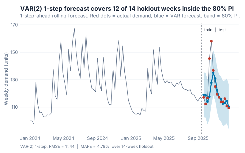
Here’s the full 104-week series, with the last 14 weeks held out as a 1-step-ahead rolling test window — the realistic weekly-replanning scenario where each Friday you forecast next Friday using everything you know so far. Before we even look at the metrics, one reassuring diagnostic: the fitted VAR(2)’s 80% prediction interval covered 12 of 14 actual values on the holdout. That’s well-calibrated for an 80% nominal level — the model is not just accurate, its uncertainty estimates are honest.
The modelling workflow, in the fable ecosystem, is absurdly compact. The business end is a single family of one-liners — one per candidate lag order, with a deterministic trend added so the AR coefficients don’t have to absorb the gentle upward drift in demand:
fits <- train |>
  model(
    lag1 = VAR(vars(demand, price, promo) ~ AR(1) + trend()),
    lag2 = VAR(vars(demand, price, promo) ~ AR(2) + trend()),
    # ... through lag8
  )
You hand VAR() the three series, fit orders 1 through 8, and let an information criterion pick the winner. Here’s where a small modelling choice genuinely matters: AIC and BIC disagree. AIC bottoms out at lag 3 (364.15); BIC bottoms out at lag 2 (459.97), with lag 3 a close second (460.32). I went with BIC — p = 2 — for three reasons, and they’re worth spelling out because this is exactly the lag-selection dilemma you’ll hit on your own data:
- Sample size. With 90 training weeks and three lagged regressors per variable per equation (9 total at p = 3, plus an intercept and trend term), AIC notoriously under-penalises complexity. BIC’s heavier penalty is the standard recommendation for VAR lag selection in small samples.
- Stationarity. At p = 2, the model’s internal dynamics decay cleanly — a shock works its way through the system and then fades, rather than building up forever. (The technical check is the largest eigenvalue of the VAR companion matrix: it comes out to 0.85, comfortably below 1. Higher lag orders nudge it closer to 1, and an almost-unit-root VAR produces IRFs that drift instead of decay.)
- Parsimony for interpretability. A VAR(2) has 2 × 3² = 18 AR coefficients to interpret. A VAR(3) has 27. If you’re showing this to a commercial director, 18 is hard enough.
VAR vs Univariate ETS — The Covariate Dividend
To measure whether those covariates actually earn their keep, I fit a plain univariate ETS on weekly demand alone — the default demand-planning baseline. Same 14-week holdout. Same 1-step-ahead rolling protocol.
One upfront note: this is a simulated teaching example. Real hospital or retail data comes with messier external shocks than any simulation can fake. What it can show is where the covariate dividend comes from and how sensitive it is to lag-selection choices — the transferable part. Here’s the side-by-side:
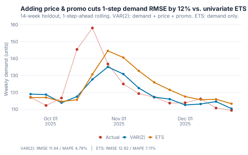
The numbers, across every loss function you’d sensibly measure:
| Model | RMSE | MAPE | MAE | Notes |
|---|---|---|---|---|
| Univariate ETS (demand only) | 12.92 | 7.11% | 9.34 | No covariates. The demand-planning default. |
| VAR(2) (demand + price + promo) | 11.44 | 4.79% | 6.56 | Same demand series, plus two covariates. |
| Improvement | 11.5% | 32.6% | 29.7% | From covariates alone, same algorithm family. |
No feature engineering. No neural networks. No foundation models. Just: tell the demand model what the price and promotion were doing, and forecast error drops by roughly 12% on RMSE, 30% on MAE, and a full third on MAPE. The MAPE gap is the one that would make a demand planner’s week — dropping average percentage error from 7% to under 5% is genuinely category-changing.
Why the big gap? Because our simulated data has real cross-dependencies (promo lifts demand, last week’s price drags it down) that the univariate model cannot see. The UC San Diego hospital data behaved similarly for the same structural reason — hospital census and surgical activity genuinely drive boarding patients, and a model that sees them beats a model that doesn’t. When the covariates are real and material, VAR dominates. When they’re not, it won’t. This is an empirical question you should always test on your own data.
Reading the Output Without Eigenvalues
Every VAR output looks like a wall of coefficients at first. Forget the table. What you actually want is the impulse response function (IRF) — a plot that answers one concrete, executive-friendly question: „If I shock price by +20% right now, what does demand do over the next 8 weeks?“
This is the part that makes VAR uniquely useful for supply chain. You can simulate a price hike of 20% (about +$1.83 on the mean price of $9.15 in our dataset), watch the cascade propagate through the system, and read the decision straight off the chart.
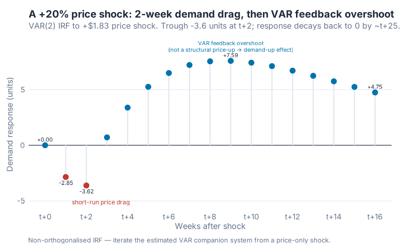
Read it left-to-right. Week 0 is the shock. Week 1: demand softens by roughly 2.9 units. Week 2 is the deepest dip, about −3.6 units below baseline — on a series whose mean runs around 125 units a week, that’s just under a 3% demand hit. That’s the structural price-drag signal the model learned during training. From week 3 onwards, the demand response turns positive and rises — but that’s not „higher prices lifting demand later.“ That’s the VAR’s own feedback dynamics producing a transient overshoot as the estimated system oscillates back to equilibrium. With the largest eigenvalue of the companion matrix at 0.85, the overshoot eventually decays to zero; it just takes longer than the 8 weeks this chart shows. Bottom line: trust the first two weeks as a pricing signal, treat the positive overshoot as model mechanics.
Why this matters for your P&L. A 3% demand hit is not academic. Scale the IRF to a category doing 10,000 units a week: the week-1 dip is about 230 units, the week-2 dip about 290 — call it 500 units of missed sell-through across the two weeks following a price move. Depending on your business, that’s a markdown clearance event, a storage cost spike, or — on the other side of the same coin — a stock-out cascade if the price move was in the other direction and you didn’t replenish to meet the lift. These are the phone calls from commercial you don’t want to be taking on a Monday morning. The IRF gives you the week-by-week number you need to plan for them before the pricing decision gets made.
That is the unique value IRFs add over a black-box model. You can draw the picture, show it to a commercial director, quantify the two-week demand-and-inventory swing the pricing move will cost, and walk out with a decision you can defend by Friday.
Where VAR Breaks
I’d be selling you fairy dust if I didn’t list the limits. Three real ones:
1. Stationarity assumption. Classical VAR wants every series to be stationary — meaning its statistical properties (mean, variance) don’t drift over time. Demand rarely obliges. In practice you difference the series — forecast week-over-week changes rather than levels — or include a deterministic trend term (as we did here) to soak up the drift. fable::VAR() handles a lot of this for you, but it’s not magic: feed it a wildly trending series without any of this care and it will still misbehave.
2. Curse of dimensionality. A VAR with k series and p lags has k²p coefficients to estimate. Three series with four lags is 36 coefficients — fine. Ten series with eight lags is 800 coefficients and you’ll overfit a desert. VAR is for small, theory-informed groups of series. For 500 SKUs, use hierarchical reconciliation or a global ML model. This is why the hospital study used three covariates, not thirty.
3. Lag-order selection matters — a lot. Pick p too small and you miss the cross-dependency. Too big and you overfit. This is why AIC/BIC information criteria exist, and why you should always cross-validate. The convenient bit is that fable does this for you automatically. The inconvenient bit is that if AIC and BIC disagree, the honest answer is usually „try both, and trust the one that wins on held-out data.“
When to Use What — A Decision Cheat Sheet
Put everything on a single shelf:
- Univariate ETS or Holt-Winters — one stable demand series, no usable covariates, and you need a forecast by lunch. The correct default 80% of the time.
- VAR — 2–6 related series (demand + price + promo + maybe competitor or weather) that you believe drive each other, and you want interpretability for the S&OP meeting. The sweet spot for category-level planning.
- XGBoost or global ML — a hierarchy, many series (50+), and rich features (hundreds of SKUs × weather × holidays × promotions). The M5-winning pattern. See our XGBoost walkthrough.
- Foundation models (TimesFM, Chronos, Lag-Llama) — fascinating research, not yet operational. Revisit in 2027. Or when you see a peer-reviewed prospective study where one actually wins. (We’re still waiting.)
The UC San Diego paper is not a sweeping condemnation of foundation models. It’s a reminder that benchmarks are cheap and deployments are expensive. Until the foundation model beats your baseline on your data, in your regime, the boring multivariate model is the honest default.
Interactive Dashboard
Before you scroll to the code, spend three minutes with the interactive explorer below. Three KPI cards up top give you the 3-second takeaway: VAR’s week-ahead forecast, the ETS baseline’s week-ahead forecast, and the +11.5% RMSE gain from adding price and promo covariates. From there, slide the lag order from 1 to 8 and watch AIC and BIC move across the candidate models — the exact disagreement (AIC prefers p = 3, BIC prefers p = 2) described in the walkthrough above. Fire a ±20% price shock and watch the IRF plot redraw live. Compare VAR against the ETS baseline at any horizon from 1 to 12 weeks. Every number in the dashboard comes straight from the R script below — nothing fabricated, nothing rounded.
Interactive Dashboard
Explore the data yourself — adjust parameters and see the results update in real time.
If you made it this far: the fact that you read a 2,000-word blog post about a 45-year-old econometric technique already tells me you’re the right kind of person for this newsletter. Welcome.
Show R Code
# =============================================================================
# generate_var_images.R — Vector Autoregression (VAR) Blog Post
# =============================================================================
# Fits fable::VAR() across lag orders 1-8 (with a deterministic trend), selects
# the best by BIC, benchmarks against a univariate ETS baseline using
# 1-step-ahead rolling forecasts on the 14-week holdout, and produces three
# 800-px static charts.
#
# Run from project root:  Rscript Scripts/generate_var_images.R
# =============================================================================

source("Scripts/theme_inphronesys.R")

suppressPackageStartupMessages({
  library(fpp3)
  library(ggplot2); library(dplyr); library(tidyr); library(scales)
  library(patchwork); library(jsonlite)
})

set.seed(42)
n <- 104

# -- 1. Simulate a realistic weekly SCM dataset (104 weeks = 2 years) ----------
promo <- rbinom(n, size = 1, prob = 0.18)

price <- numeric(n); price[1] <- 10
for (i in 2:n) {
  price[i] <- 0.80 * price[i - 1] + 0.20 * 10 +
              rnorm(1, 0, 0.10) - 0.80 * promo[i]
  price[i] <- max(7.5, price[i])
}

demand <- numeric(n); demand[1] <- 100; demand[2] <- 100
for (i in 3:n) {
  trend_c <- 0.15 * i
  seas_c  <- 6 * sin(2 * pi * i / 52 - pi / 2)
  price_c <- -8.0 * (price[i - 1] - 10)
  promo_c <- 30 * promo[i]
  ar_c    <- 0.30 * (demand[i - 1] - (100 + 0.15 * (i - 1)))
  demand[i] <- 100 + trend_c + seas_c + price_c + promo_c + ar_c +
               rnorm(1, 0, 1.8)
}

dates <- as.Date("2024-01-01") + (0:(n - 1)) * 7
tsbl <- as_tsibble(
  tibble::tibble(
    week = yearweek(dates),
    demand = round(demand, 1), price = round(price, 3),
    promo_intensity = as.numeric(promo)
  ),
  index = week
)

# -- 2. Train / test split (90 / 14) -------------------------------------------
n_train <- 90
train <- tsbl %>% slice_head(n = n_train)
test  <- tsbl %>% slice_tail(n = n - n_train)

# -- 3. Fit VAR at lag orders 1-8 (with deterministic trend), pick min-BIC -----
# The trend() term keeps the AR coefficients from absorbing the demand drift —
# crucial for a stable IRF. BIC is the standard lag-selection criterion for VAR
# in small samples (AIC under-penalises complexity; AICc becomes unreliable
# when parameter count approaches n).
fits_var <- train %>%
  model(
    lag1 = VAR(vars(demand, price, promo_intensity) ~ AR(1) + trend()),
    lag2 = VAR(vars(demand, price, promo_intensity) ~ AR(2) + trend()),
    lag3 = VAR(vars(demand, price, promo_intensity) ~ AR(3) + trend()),
    lag4 = VAR(vars(demand, price, promo_intensity) ~ AR(4) + trend()),
    lag5 = VAR(vars(demand, price, promo_intensity) ~ AR(5) + trend()),
    lag6 = VAR(vars(demand, price, promo_intensity) ~ AR(6) + trend()),
    lag7 = VAR(vars(demand, price, promo_intensity) ~ AR(7) + trend()),
    lag8 = VAR(vars(demand, price, promo_intensity) ~ AR(8) + trend())
  )

gl <- glance(fits_var) %>% arrange(.model)
chosen_lag <- as.integer(sub("lag", "", gl$.model[which.min(gl$BIC)]))
#> AIC by lag: 437.15, 385.65, 364.15, 366.89, 378.09, 380.46, 385.68, 387.05
#> BIC by lag: 496.87, 459.97, 460.32, 484.70, 517.32, 540.90, 567.09, 589.21
#> AIC minimised at p = 3 (364.15); BIC minimised at p = 2 (459.97), p = 3 close second (460.32)
#> chosen_lag: 2

# -- 4. Univariate ETS baseline on demand --------------------------------------
fit_ets <- train %>% model(ets = ETS(demand))

# -- 5. Manual VAR fit (equation-by-equation OLS) for IRF + rolling forecasts --
# Design matrix includes constant + linear trend + p*3 lag columns, matching
# the fable spec so the closed-form coefficient matrices A_1..A_p are directly
# usable for iterating the IRF companion system.
Y <- as.matrix(train %>% as_tibble() %>%
                 select(demand, price, promo_intensity))
p <- chosen_lag
T_obs <- nrow(Y)
X_reg <- matrix(0, nrow = T_obs - p, ncol = 2 + p * 3)
X_reg[, 1] <- 1
X_reg[, 2] <- (p + 1):T_obs            # deterministic trend
for (lag_i in 1:p) {
  X_reg[, (3 + (lag_i - 1) * 3):(2 + lag_i * 3)] <-
    Y[(p - lag_i + 1):(T_obs - lag_i), ]
}
Y_reg <- Y[(p + 1):T_obs, ]
B <- solve(crossprod(X_reg), crossprod(X_reg, Y_reg))
A_mats <- lapply(1:p,
  function(i) t(B[(3 + (i - 1) * 3):(2 + i * 3), ]))

# Sanity-check stationarity: largest-modulus eigenvalue of the VAR companion
# matrix must be < 1 for a stable (trend-stationary) fit.
k <- 3
companion <- matrix(0, nrow = k * p, ncol = k * p)
for (lag_i in 1:p) {
  companion[1:k, ((lag_i - 1) * k + 1):(lag_i * k)] <- A_mats[[lag_i]]
}
if (p > 1) companion[(k + 1):(k * p), 1:(k * (p - 1))] <- diag(1, k * (p - 1))
max_mod_root <- max(Mod(eigen(companion)$values))   # should be < 1

# -- 6. 1-step-ahead rolling forecasts on the 14-week holdout ------------------
Y_all <- as.matrix(tsbl %>% as_tibble() %>%
                     select(demand, price, promo_intensity))
n_test <- nrow(test)
var_1step <- matrix(NA_real_, nrow = n_test, ncol = 3)
for (k in 1:n_test) {
  t_k <- n_train + k
  x <- c(1, t_k)
  for (lag_i in 1:p) x <- c(x, Y_all[t_k - lag_i, ])
  var_1step[k, ] <- x %*% B
}

ets_full <- fit_ets %>% refit(tsbl, reestimate = FALSE)
ets_pred <- augment(ets_full) %>% slice_tail(n = n_test) %>% pull(.fitted)

# -- 7. Holdout accuracy (1-step rolling) --------------------------------------
actual <- test$demand
rmse <- function(y, yhat) sqrt(mean((y - yhat)^2))
mape <- function(y, yhat) mean(abs((y - yhat) / y)) * 100
mae  <- function(y, yhat) mean(abs(y - yhat))

cat(sprintf("VAR(%d)  RMSE = %.2f   MAPE = %.2f%%   MAE = %.2f\n",
            chosen_lag, rmse(actual, var_1step[, 1]),
            mape(actual, var_1step[, 1]), mae(actual, var_1step[, 1])))
cat(sprintf("ETS     RMSE = %.2f   MAPE = %.2f%%   MAE = %.2f\n",
            rmse(actual, ets_pred), mape(actual, ets_pred),
            mae(actual, ets_pred)))
#> VAR(2)  RMSE = 11.44   MAPE = 4.79%   MAE = 6.56
#> ETS     RMSE = 12.92   MAPE = 7.11%   MAE = 9.34

# -- 8. Impulse response: +20% price shock -------------------------------------
H_IRF <- 8
price_mean <- mean(Y[, "price"])
shock_size <- 0.20 * price_mean   # ≈ +$1.83

y_hist <- matrix(0, nrow = H_IRF + p, ncol = 3)
colnames(y_hist) <- c("demand", "price", "promo_intensity")
shock_row <- p
y_hist[shock_row, "price"] <- shock_size

irf <- numeric(H_IRF + 1)
for (h in 1:H_IRF) {
  y_next <- numeric(3)
  for (lag_i in 1:p) {
    y_next <- y_next + A_mats[[lag_i]] %*% y_hist[shock_row + h - lag_i, ]
  }
  y_hist[shock_row + h, ] <- y_next
  irf[h + 1] <- y_next[1]
}
#> demand response at t+1..t+8 (units):
#>   -2.86, -3.62, +0.71, +3.38, +5.25, +6.49, +7.21, +7.55

# Charts 1-3 (forecast-vs-actual, VAR vs ETS, IRF) follow — standard ggplot
# using theme_inphronesys() for the brand styling.
References
[^1]: Poursoltan, L. et al. (2025). Prospective comparison of econometric, machine learning, and foundation models for forecasting emergency department boarding patients. npj Health Systems, vol. 2, article 49. DOI: 10.1038/s44401-025-00054-z. Open access.
[^2]: Sims, C. A. (1980). Macroeconomics and Reality. Econometrica, 48(1), 1–48.
Schreibe einen Kommentar