Gradient-boosted trees like XGBoost have become the default ML choice for multi-series forecasting — not because they beat classical methods by huge margins, but because they scale across hundreds of SKUs and let you fold in real covariates (promotions, holidays, prices) that ETS and SNAIVE can’t touch. This post is a hands-on walkthrough: we apply the same family of techniques popularised by M5-era gradient-boosted models to a classic public dataset (Walmart weekly sales), and honestly measure where the complexity earns its keep — and where it doesn’t.
It’s the practical follow-up to two earlier posts in this series: The M5 Lesson explained why gradient-boosted trees won the biggest forecasting competition ever run; The Horse Race showed how to pick a forecasting winner with MASE and cross-validation. Today is the how — and specifically how in R, with the tidymodels + modeltime stack.
The Dataset: Walmart Weekly Sales
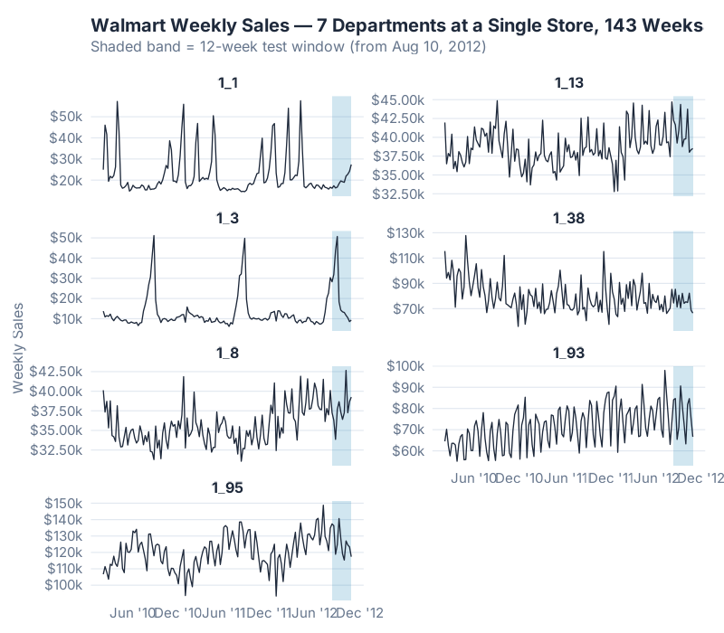
Our example is timetk::walmart_sales_weekly — a public sample distributed with the timetk R package, originally released for the 2014 Walmart Recruiting Kaggle competition. It contains 7 departments at a single Walmart store across 143 weeks (February 2010 to October 2012). Think of each series as a product category in one store: apparel, grocery, electronics, and so on. It’s a convenient teaching example for end-to-end ML forecasting — retail, weekly, multi-series, with a real holiday covariate baked in — without the operational weight of a production-scale dataset.
That last point matters more than it looks. Most demand series come with context: promotions, holidays, price changes, weather. Classical statistical models like ETS and SNAIVE can’t use any of it — they see only the sales number. Machine learning models can use everything you hand them, which is why they tend to pull ahead on rich retail data and stay even on sparse industrial data.
The IsHoliday flag in this dataset captures exactly the kind of event that theoretically breaks a naive forecaster: Thanksgiving, Black Friday, Christmas week. A model that knows „next week is a holiday week“ has an advantage over a model that doesn’t — at least in principle. Whether it actually helps in practice on this particular dataset is a question we’ll return to in the Feature Importance section, and the answer may surprise you.
We train on the first 131 weeks and hold out the last 12 weeks (from August 10, 2012 onward) as the test window — a realistic quarter-ahead forecasting horizon.
Why Feature Engineering Is Everything
Here is the one thing that trips up everyone new to ML forecasting: XGBoost has no idea it is looking at time series data.
ETS knows. Its equations explicitly encode level, trend, and seasonality — that’s literally what the letters stand for. SNAIVE knows — its entire method is „what happened one season ago.“ These models come pre-wired to recognise the rhythm of demand.
XGBoost doesn’t. To XGBoost, every row is an independent observation, every column just a number. It has no concept of „last week“ or „same week last year“ unless you explicitly build a column called lag_52 and hand it over. If you don’t, the model cannot learn annual seasonality — not because it isn’t smart enough, but because the information literally isn’t in its input.
Think of it like this: ETS is a specialist who has memorised the seasonal calendar. XGBoost is a brilliant generalist who can learn anything — but only if you point at it. Feature engineering is the pointing.
This is why the M5 winners talked about features, not algorithms. Everyone at the top of the leaderboard used gradient-boosted trees. The difference between rank 1 and rank 1,000 was how thoughtfully each team had translated demand history into tabular columns the model could read.
Building the Feature Engineering Recipe
Our feature pipeline adds a specific kind of column for each thing we want the model to see. Crucially, every lag and rolling feature is computed strictly from the past (t-n through t-1, never including t), and computed per department so a high-volume category can’t leak its numbers into a low-volume one.
1. Lag features (1, 4, 13, 26, 52 weeks). These capture memory at different horizons:
lag_1— last week’s sales. Short-term momentum.lag_4— one month ago. Captures the monthly cycle.lag_13— one quarter. Quarterly rhythm.lag_26— half-year. Seasonal mid-point.lag_52— same week last year. The annual anchor.
2. Rolling window features (4w, 13w, 26w means; 4w standard deviation). These smooth out the noise:
- 4-week rolling mean — the recent trajectory.
- 13-week rolling mean — the quarterly level.
- 26-week rolling mean — the long-run baseline.
- 4-week rolling sd — local volatility, which helps the model calibrate its response on noisier series.
3. Calendar features (month, quarter, week-of-year, year). Time-stamp derivatives (via step_timeseries_signature()) that let the model pick up structural patterns like „week 47 is always Black Friday.“
4. The IsHoliday covariate. Pre-built into the dataset. This is the feature ETS and SNAIVE cannot use — at least in principle. Whether it earns its keep on a given dataset is an empirical question, and on this one the answer is not what you’d expect.
5. Department identity dummies. One-hot encoded series IDs. These are what turn this into a global model — one model fit across all 7 departments, with department identity as just another feature. The model learns the shared structure (everyone spikes at Christmas) while still letting each department have its own intercept.
A small sketch of what the transformation does:
| Raw columns | → | Engineered feature columns |
|---|---|---|
Date, Sales, Dept_ID, IsHoliday |
→ | lag_1, lag_4, lag_13, lag_26, lag_52, roll_mean_4, roll_mean_13, roll_mean_26, roll_sd_4, month, quarter, week, year, IsHoliday, id_1_1…id_1_95 |
Four columns in. Twenty-plus columns out. XGBoost gets to pick which of them actually matter — and as we’ll see, its choices are not what you’d expect.
Training the Global Model
The tidymodels + modeltime stack lets a machine-learning model and a statistical model compete on the same footing. The workflow — stripped to its essentials:
# Feature engineering recipe — lag/rolling features are computed upstream
# per department (strictly past-window only) to prevent cross-series leakage
recipe_xgb <- recipe(Weekly_Sales ~ ., data = train_feat) %>%
  step_timeseries_signature(Date) %>%
  step_dummy(all_nominal_predictors()) %>%
  step_naomit(all_predictors())

# XGBoost spec
xgb_spec <- boost_tree(
  trees = 500, min_n = 10, tree_depth = 6,
  learn_rate = 0.01, sample_size = 0.8
) %>% set_engine("xgboost") %>% set_mode("regression")

# Fit globally — one model, all 7 departments
fit_xgb <- workflow() %>%
  add_recipe(recipe_xgb) %>%
  add_model(xgb_spec) %>%
  fit(data = train_feat)
Three things worth flagging:
- One model, all 7 departments.
fit()receives the entire panel, not seven per-series datasets. The department dummies carry the identity. This „global model“ approach is the single biggest architectural difference between M5-style ML forecasting and classical one-series-at-a-time ETS. - The recipe runs inside the workflow. Feature engineering is versioned with the model, not a separate script. When you
predict()on new data, the same transformations replay automatically. - No hand-tuning for the first pass. We use sensible defaults (500 trees, depth 6, learn rate 0.01). A small 3×3 hyperparameter grid later shows the best combination we found (depth 9, learn rate 0.01) is only 2–4% better than this shipping spec (depending on whether we compare against the main fit or the same-spec cell inside the grid) — the features are doing the real work, not the knobs.
The full reproducible script — including the per-department lag generation and the baseline fits — is in the collapsible section at the bottom of this post.
Results: The Model Comparison
We now run three models on the 12-week test window:
- XGBoost — one global model across all 7 departments.
- ETS — one model per department, via
forecast::stlf()(STL decomposition + ETS on the seasonally-adjusted series). Plainforecast::ets()caps its seasonal period at 24, so for weekly data (m = 52)stlf()is the forecast package’s recommended path. It is a strong benchmark, not a handicapped one. - SNAIVE — one model per department. „This week next year = this week last year.“ Our floor.
We score them with MASE. A MASE of 1.0 means „my forecast errors are about the same size as a seasonal-naive forecast on the training history.“ Below 1.0 is better than last-year-ago naive; above 1.0 is worse. Winner per row is bold.
| Department | XGBoost | ETS | SNAIVE |
|---|---|---|---|
| 1_1 | 0.547 | 0.327 | 0.318 |
| 1_3 | 5.685 | 6.105 | 6.166 |
| 1_8 | 0.433 | 0.655 | 2.044 |
| 1_13 | 0.831 | 0.820 | 1.062 |
| 1_38 | 0.516 | 0.603 | 0.635 |
| 1_93 | 0.588 | 0.516 | 0.709 |
| 1_95 | 0.748 | 0.935 | 0.757 |
| Overall mean | 1.336 | 1.423 | 1.670 |
| Median | 0.588 | 0.655 | 0.757 |
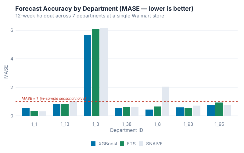
XGBoost wins on mean MASE — 1.336 versus ETS at 1.423, a 6.1% improvement. It beats SNAIVE by 20%. Those are real gains, but they are not a revolution: per-department, the three models trade blows. XGBoost takes four departments outright (1_3, 1_8, 1_38, 1_95). ETS takes two (1_13, 1_93). And on department 1_1, neither of them beats SNAIVE.
Two results in this table deserve their own paragraphs, because they are where the interesting supply chain lessons live.
Department 1_3 is where MASE itself becomes the story. All three MASE values are around 6 — which looks catastrophic until you look at the raw series. The August spike from ~$10k baseline to above $50k is not unprecedented: it’s an annual event. The series spiked to $51,159 on 2010-08-27 and $49,776 on 2011-08-26, both in training, before the 2012-08-31 spike of $50,701 in the test window. The models mis-time and mis-magnitude the spike by enough that MASE — which scales against a tiny in-sample SNAIVE denominator on an otherwise very regular series — balloons to ~6. The supply-chain lesson still holds: flag it, raise an alert, don’t auto-post. But the reason isn’t that the spike was unprecedented. It’s that MASE is unforgiving when your baseline series is predictable and your forecast misses the one event that matters. Excluding 1_3, the XGBoost mean drops to 0.61, ETS to 0.64, SNAIVE to 0.92.
Department 1_8 is where feature engineering pays off.
XGBoost: MASE 0.43 | SNAIVE: MASE 2.04 — a 79% reduction in forecast error.
This is the one department where the model’s memory features clearly outperform naive seasonality, because 1_8’s history has a repeatable week-to-week structure that SNAIVE’s once-a-year lookup misses entirely. When people talk about ML beating naive forecasting by „huge margins,“ they’re usually describing a series like 1_8. The honest caveat is that most of your SKUs won’t look like 1_8 — they’ll look like 1_1.
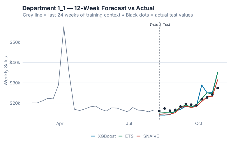
Department 1_1 is the humility pill. Its final 12 weeks happened to land almost exactly on top of the same 12 weeks from the previous year — which is SNAIVE’s entire method. A 500-tree gradient-boosted model that has seen every other department’s history cannot beat a one-line formula that just looks up the past, because there’s nothing left to beat. The forecast-vs-actual chart above is Department 1_1, and you can see all three models converging on roughly the same answer — that’s the point. On a series where last-year is right, ML can only match; it cannot improve.
The good news in the table is consistency against SNAIVE: XGBoost beats SNAIVE on 6 of 7 departments — the only miss is Department 1_1. The honest news is that „6.1% better than ETS on the mean, 10.2% better on the median“ is the real magnitude of the ML advantage on this kind of data. Budget your expectations accordingly.
Feature Importance: What the Model Actually Learned
Feature importance answers the question every stakeholder asks: what is the model actually using to make predictions? XGBoost’s „Gain“ metric measures how much each feature contributed to reducing the training loss across all splits it appeared in.
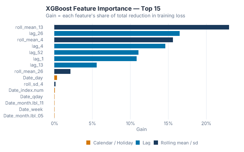
The ranking confirms a pattern consistently observed across ML forecasting studies (see Januschowski et al. 2022 for a review of tree-based forecasting): memory features dominate. The most important feature is roll_mean_13 — the 13-week trailing average — at 23.0% of total Gain. lag_26 (six months ago) is second at 16.5%. roll_mean_4 is third at 15.6%. lag_4 is fourth at 14.6%. lag_52 — the „same week last year“ feature we spent the most time building intuition around — comes in at only fifth place, 11.1% of Gain. Add lag_1 (10.8%) and the top six features alone account for over 91% of everything the model learned.
A Known Pattern, Reconfirmed: IsHoliday Didn’t Crack the Top 15
Here is what you’ll find when you inspect the feature importance table: the holiday flag contributed nothing measurable to the model. IsHoliday didn’t rank in the top 15 features. None of the calendar features (week-of-year, month, quarter, year) contributed more than half a percent of Gain each. On a dataset where Thanksgiving, Black Friday, and Christmas should — in theory — be exactly the kind of event a covariate helps with, the model quietly ignored the label we gave it. This isn’t novel: it’s a recurring pattern in the ML forecasting literature. Once your history covers two or more seasonal cycles, lag features tend to absorb the signal that calendar indicators were meant to carry.
Why? Because lag_52 got there first. „Sales in the same week of last year“ already encodes every recurring event on the calendar. Thanksgiving week 2012’s best predictor isn’t a boolean IsHoliday = 1; it’s the actual sales number from Thanksgiving week 2011, which is exactly what lag_52 carries. By the time XGBoost considered IsHoliday, the seasonal signal had been fully absorbed by the lag and rolling features. Adding a flag to mark „this is a holiday“ was redundant with a feature that already said „last year in this exact week, we sold $X.“
The lesson for your own feature engineering: lags eat calendar features for breakfast, as long as your history is long enough for a full seasonal cycle. If you only have 18 months of data, lag_52 isn’t available for the first year, and IsHoliday might genuinely earn its keep. With two full cycles, the covariate usually becomes decorative.
In supply chain terms: the features that moved the needle were memory, not context. The model’s most predictive inputs are „the smoothed 13-week level,“ „sales six months ago,“ and „the smoothed one-month level.“ Raw year-ago values helped, but smoothed windows helped more — because the rolling means filter out the week-to-week noise that a single lag carries. The M5 lesson still holds: feature engineering is the whole story. On this data, the story is specifically about lag and rolling-window engineering. Calendar engineering turned out to be optional.
The Honest Verdict: When XGBoost Beats ETS at SKU Level
The headline finding: single-digit-percent improvements are the norm for ML forecasters on multi-series retail data, not the exception. The M5 Lesson post covered a sobering result from the competition: at the finest hierarchy level (SKU-store, the one your ERP actually plans against), the M5 winner beat the strongest classical benchmark by only about 3%. Not 30%. Not 300%. Single digits.
Our walkthrough here lands in the same broad neighbourhood — XGBoost is 6.1% better than STL-ETS on mean MASE on this particular 7-department sample, 10.2% better on the median. The metrics and datasets aren’t directly comparable to M5’s WRMSSE, but the order of magnitude is consistent with what’s been reported across the ML forecasting literature on weekly retail data. Expect single-digit-percent gains, budget for the engineering effort accordingly, and don’t promise the business more than that. Anyone selling you a 40% accuracy lift from „AI forecasting“ has not actually run the benchmark.
Here is when XGBoost earns its complexity:
- You have multiple related series. Seven departments, 500 SKUs, 40 distribution centres — the global model amortises feature engineering across all of them and learns shared structure. A single isolated series is ETS territory.
- You have real covariates that actually move demand. Promotion calendars, price changes, weather, or holiday flags with genuinely different magnitude than non-holiday weeks. If
IsHolidaybarely moves your series (as we found here), the covariate advantage evaporates. - You have enough history. Two full seasonal cycles is the minimum. Below that, there aren’t enough
lag_52observations for the model to learn the annual anchor, and XGBoost collapses onto short-term memory. - Your series have heterogeneous structure. Different products with different seasonality, different trend directions, different volatility regimes. XGBoost handles this natively via series dummies; fitting 500 separate ETS models is slow and brittle.
And here is when ETS (or even SNAIVE) will quietly beat you:
- Single isolated series. No cross-learning advantage to exploit.
- Short history. Under two full seasonal cycles, lag features go to NA and the model loses its best predictor.
- Sparse intermittent demand. Spare parts, dead stock, anything with lots of zeros. Croston’s method and its descendants are purpose-built; XGBoost is not.
- The next period happens to look like last year. Department 1_1 above. SNAIVE wins and there is nothing you can do about it — which is why SNAIVE belongs in every benchmark.
The verdict: XGBoost is the right default when you have multi-series data with real demand drivers. It is the wrong default when you don’t. Don’t let anyone tell you the choice is always obvious — the whole point of running the horse race is that you can’t predict the winner.
Your Next Steps
- Run this script on your own ERP weekly data. The recipe adapts with a single column rename. If you have store/DC/SKU identifiers, one-hot encode them and go global — you’ll get an M5-style model on your own data in an afternoon.
- Segment A/B/C items before fitting globally. Mixing fast-movers with dead stock in one global model is how you get mediocre forecasts on both. Fit A-items globally, B-items globally, and handle C-items with intermittent-demand methods like Croston.
- Flag volatility outliers before you trust a forecast. Department 1_3 above is every forecaster’s nightmare — a demand regime change the model could not have seen. Calculate MASE per series and escalate anything > 2 for human review instead of auto-posting it to your plan.
- Always run SNAIVE as your benchmark before deploying anything fancier. If XGBoost can’t beat SNAIVE on a given series (Department 1_1 above), either your features are wrong, your history is too short, or the series just happens to repeat itself. Either way, you needed to know.
- Start with lag + rolling features, add calendar + covariates only when they earn their keep. On this dataset the memory features (lags and rolling windows) account for over 99% of total model Gain; the holiday flag contributed nothing. Your own data may differ — but the way you find out is empirically, not by assumption.
Interactive Dashboard
Explore the forecast comparison across all 7 Walmart departments — pick any department, toggle models, and see where XGBoost wins, where ETS stays competitive, and where 1_3’s demand spike breaks every model at once.
Interactive Dashboard
Explore the data yourself — adjust parameters and see the results update in real time.
Show R Code
# =============================================================================
# generate_xgboost_images.R
#   Part of the April 2026 Forecasting Month series
#   Blog post: "XGBoost for Supply Chain Forecasting: The Feature Engineering
#              Is the Whole Story"
#
# Produces 4 images in Images/:
#   1. xgb_walmart_series.png       — 7 Walmart departments, weekly sales, test shaded
#   2. xgb_feature_importance.png   — XGBoost top-15 features by Gain
#   3. xgb_model_comparison.png     — MASE by department × (XGBoost, ETS, SNAIVE)
#   4. xgb_forecast_vs_actual.png   — Dept 1_1: forecasts + actuals, test window
#
# Run from project root:
#   Rscript Scripts/generate_xgboost_images.R
# =============================================================================

suppressPackageStartupMessages({
  library(tidymodels)
  library(modeltime)
  library(timetk)
  library(tidyverse)
  library(xgboost)
  library(lubridate)
  library(slider)
  library(forecast)
})

source("Scripts/theme_inphronesys.R")
set.seed(42)

# ---- 1. Data -----------------------------------------------------------------
data("walmart_sales_weekly", package = "timetk")

walmart <- walmart_sales_weekly %>%
  select(id, Date, Weekly_Sales, IsHoliday) %>%
  mutate(
    id        = as.character(id),
    IsHoliday = as.integer(IsHoliday)
  ) %>%
  arrange(id, Date)

depts   <- sort(unique(walmart$id))
horizon <- 12

# Time-aware split: the last 12 distinct dates become the test window
all_dates  <- sort(unique(walmart$Date))
test_dates <- tail(all_dates, horizon)
split_date <- min(test_dates)

train_data <- walmart %>% filter(Date <  split_date)
test_data  <- walmart %>% filter(Date >= split_date)

# ---- 2. Honest feature engineering (per-id; no cross-series leakage) ---------
# Rolling mean / sd are computed over the STRICTLY PAST window (t-n..t-1).
# Lags use only past Weekly_Sales. Grouping by id prevents series-boundary bleed.
lag_roll <- function(x, n, fun = mean) {
  out <- rep(NA_real_, length(x))
  for (i in seq_along(x)) {
    if (i > n) out[i] <- fun(x[(i - n):(i - 1)], na.rm = TRUE)
  }
  out
}

add_features <- function(df) {
  df %>%
    group_by(id) %>%
    arrange(Date) %>%
    mutate(
      lag_1        = dplyr::lag(Weekly_Sales, 1),
      lag_4        = dplyr::lag(Weekly_Sales, 4),
      lag_13       = dplyr::lag(Weekly_Sales, 13),
      lag_26       = dplyr::lag(Weekly_Sales, 26),
      lag_52       = dplyr::lag(Weekly_Sales, 52),
      roll_mean_4  = lag_roll(Weekly_Sales,  4, mean),
      roll_mean_13 = lag_roll(Weekly_Sales, 13, mean),
      roll_mean_26 = lag_roll(Weekly_Sales, 26, mean),
      roll_sd_4    = lag_roll(Weekly_Sales,  4, sd)
    ) %>%
    ungroup() %>%
    mutate(id = factor(id))
}

walmart_feat <- add_features(walmart)
train_feat   <- walmart_feat %>% filter(Date <  split_date)
test_feat    <- walmart_feat %>% filter(Date >= split_date)

# ---- 3. Recipe ---------------------------------------------------------------
recipe_xgb <- recipe(Weekly_Sales ~ ., data = train_feat) %>%
  step_timeseries_signature(Date) %>%
  step_rm(contains("iso"),   contains("xts"),    contains("hour"),
          contains("minute"),contains("second"), contains("am.pm"),
          contains("mday"),  contains("yday")) %>%
  step_rm(Date) %>%
  step_normalize(Date_index.num, Date_year) %>%
  step_dummy(all_nominal_predictors(), one_hot = FALSE) %>%
  step_naomit(all_predictors())

# ---- 4. XGBoost model + workflow ---------------------------------------------
model_xgb <- boost_tree(
    trees       = 500,
    min_n       = 10,
    tree_depth  = 6,
    learn_rate  = 0.01,
    sample_size = 0.8
  ) %>%
  set_engine("xgboost") %>%
  set_mode("regression")

wf_xgb  <- workflow() %>% add_recipe(recipe_xgb) %>% add_model(model_xgb)
fit_xgb <- fit(wf_xgb, data = train_feat)

pred_xgb <- predict(fit_xgb, new_data = test_feat) %>%
  bind_cols(test_feat %>% select(id, Date, Weekly_Sales)) %>%
  rename(xgb = .pred) %>%
  mutate(id = as.character(id))

# ---- 5. Baselines: SNAIVE and ETS, fit per department ------------------------
per_dept_baselines <- map_df(depts, function(s) {
  train_s <- train_data %>% filter(id == s) %>% arrange(Date)
  test_s  <- test_data  %>% filter(id == s) %>% arrange(Date)

  y <- ts(train_s$Weekly_Sales, frequency = 52)

  sn   <- forecast::snaive(y, h = horizon)$mean
  # forecast::ets() caps seasonal period at 24, so for weekly (m = 52) we use
  # stlf(): STL decomposition + ETS on the seasonally-adjusted series.
  ets_ <- forecast::stlf(y, h = horizon, method = "ets")$mean

  tibble(
    id     = s,
    Date   = test_s$Date,
    actual = test_s$Weekly_Sales,
    snaive = as.numeric(sn),
    ets    = as.numeric(ets_)
  )
})

# ---- 6. MASE (seasonal, m = 52) ----------------------------------------------
# MASE denominator = mean(|y_t - y_{t-m}|) on the IN-SAMPLE training data.
mase <- function(actual, forecast, train_actual, m = 52) {
  denom <- mean(abs(diff(train_actual, lag = m)), na.rm = TRUE)
  mean(abs(actual - forecast), na.rm = TRUE) / denom
}

# Pre-build per-department training vectors so MASE uses the correct denominator.
train_map <- train_data %>%
  arrange(id, Date) %>%
  group_by(id) %>%
  summarise(train_vec = list(Weekly_Sales), .groups = "drop")

scores <- per_dept_baselines %>%
  left_join(pred_xgb %>% select(id, Date, xgb), by = c("id", "Date")) %>%
  left_join(train_map, by = "id") %>%
  group_by(id) %>%
  summarise(
    mase_xgb    = mase(actual, xgb,    train_vec[[1]], 52),
    mase_ets    = mase(actual, ets,    train_vec[[1]], 52),
    mase_snaive = mase(actual, snaive, train_vec[[1]], 52),
    .groups = "drop"
  )

mean_mase <- scores %>%
  summarise(
    XGBoost = mean(mase_xgb),
    ETS     = mean(mase_ets),
    SNAIVE  = mean(mase_snaive)
  )

# ---- 7. Feature importance ---------------------------------------------------
importance <- xgboost::xgb.importance(model = extract_fit_engine(fit_xgb)) %>%
  as_tibble()

top15 <- importance %>%
  arrange(desc(Gain)) %>%
  slice_head(n = 15) %>%
  mutate(
    feature_type = case_when(
      str_detect(Feature, "^lag_")         ~ "Lag",
      str_detect(Feature, "^roll")         ~ "Rolling mean / sd",
      str_detect(Feature, "(?i)holiday")   ~ "Calendar / Holiday",
      str_detect(Feature, "^Date_")        ~ "Calendar / Holiday",
      str_detect(Feature, "^id_")          ~ "Series ID",
      TRUE                                 ~ "Other"
    )
  )

# ---- 8. Images ---------------------------------------------------------------

# --- 8.1 Walmart weekly series, faceted, test shaded ---
test_shade <- tibble(
  xmin = split_date, xmax = max(walmart$Date),
  ymin = -Inf,       ymax = Inf
)

p1 <- ggplot(walmart, aes(x = Date, y = Weekly_Sales)) +
  geom_rect(data = test_shade,
            aes(xmin = xmin, xmax = xmax, ymin = ymin, ymax = ymax),
            fill = iph_colors$blue, alpha = 0.18, inherit.aes = FALSE) +
  geom_line(color = iph_colors$dark, linewidth = 0.45) +
  facet_wrap(~ id, ncol = 2, scales = "free_y") +
  scale_x_date(date_breaks = "6 months", date_labels = "%b '%y") +
  scale_y_continuous(labels = scales::dollar_format(scale = 1e-3, suffix = "k")) +
  labs(title    = "Walmart Weekly Sales — 7 Departments, 143 Weeks",
       subtitle = sprintf("Shaded band = 12-week test window (from %s)",
                          format(split_date, "%b %d, %Y")),
       x = NULL, y = "Weekly Sales") +
  theme_inphronesys(grid = "y")

ggsave("https://inphronesys.com/wp-content/uploads/2026/04/xgb_walmart_series-2.png", p1,
       width = 8, height = 7, dpi = 100, bg = "white")

# --- 8.2 Feature importance bar chart ---
feature_colors <- c("Lag"                = iph_colors$blue,
                    "Rolling mean / sd"  = iph_colors$navy,
                    "Calendar / Holiday" = iph_colors$orange,
                    "Series ID"          = iph_colors$teal,
                    "Other"              = iph_colors$grey)

p2 <- ggplot(top15, aes(x = Gain, y = reorder(Feature, Gain), fill = feature_type)) +
  geom_col(width = 0.75) +
  scale_fill_manual(values = feature_colors, name = NULL) +
  scale_x_continuous(labels = scales::percent_format(accuracy = 1)) +
  labs(title    = "XGBoost Feature Importance — Top 15",
       subtitle = "Gain = each feature's share of total reduction in training loss",
       x = "Gain", y = NULL) +
  theme_inphronesys(grid = "x")

ggsave("https://inphronesys.com/wp-content/uploads/2026/04/xgb_feature_importance-2.png", p2,
       width = 8, height = 5, dpi = 100, bg = "white")

# --- 8.3 MASE comparison (grouped bars) ---
mase_long <- scores %>%
  pivot_longer(starts_with("mase_"), names_to = "model", values_to = "mase") %>%
  mutate(model = recode(model,
                        mase_xgb    = "XGBoost",
                        mase_ets    = "ETS",
                        mase_snaive = "SNAIVE"),
         model = factor(model, levels = c("XGBoost", "ETS", "SNAIVE")))

p3 <- ggplot(mase_long, aes(x = id, y = mase, fill = model)) +
  geom_col(position = position_dodge(0.8), width = 0.72) +
  geom_hline(yintercept = 1, linetype = "dashed",
             color = iph_colors$red, linewidth = 0.5) +
  annotate("text", x = 0.6, y = 1,
           label = "MASE = 1  (in-sample seasonal naive)",
           hjust = 0, vjust = -0.6,
           color = iph_colors$red, size = 3.2, fontface = "italic",
           family = "Inter") +
  scale_fill_manual(values = c("XGBoost" = iph_colors$blue,
                               "ETS"     = iph_colors$green,
                               "SNAIVE"  = iph_colors$lightgrey),
                    name = NULL) +
  labs(title    = "Forecast Accuracy by Department (MASE — lower is better)",
       subtitle = "12-week holdout across 7 Walmart departments",
       x = "Department ID", y = "MASE") +
  theme_inphronesys(grid = "y")

ggsave("https://inphronesys.com/wp-content/uploads/2026/04/xgb_model_comparison-2.png", p3,
       width = 8, height = 5, dpi = 100, bg = "white")

# --- 8.4 Dept 1_1: context + forecasts vs actual ---
dept_focus    <- "1_1"
context_weeks <- 24

context_df <- train_data %>%
  filter(id == dept_focus) %>%
  arrange(Date) %>%
  slice_tail(n = context_weeks)

forecast_df <- per_dept_baselines %>%
  filter(id == dept_focus) %>%
  left_join(pred_xgb %>% select(id, Date, xgb), by = c("id", "Date")) %>%
  pivot_longer(c(xgb, ets, snaive), names_to = "model", values_to = "forecast") %>%
  mutate(model = recode(model, xgb = "XGBoost", ets = "ETS", snaive = "SNAIVE"),
         model = factor(model, levels = c("XGBoost", "ETS", "SNAIVE")))

actuals_df <- per_dept_baselines %>%
  filter(id == dept_focus) %>%
  select(Date, actual)

p4 <- ggplot() +
  geom_line(data = context_df, aes(x = Date, y = Weekly_Sales),
            color = iph_colors$grey, linewidth = 0.55) +
  geom_vline(xintercept = split_date,
             linetype = "dashed", color = iph_colors$dark, linewidth = 0.4) +
  geom_line(data = forecast_df,
            aes(x = Date, y = forecast, color = model),
            linewidth = 0.9) +
  geom_point(data = actuals_df,
             aes(x = Date, y = actual),
             color = iph_colors$dark, size = 2.2) +
  scale_color_manual(values = c("XGBoost" = iph_colors$blue,
                                "ETS"     = iph_colors$green,
                                "SNAIVE"  = iph_colors$red), name = NULL) +
  scale_y_continuous(labels = scales::dollar_format(scale = 1e-3, suffix = "k")) +
  labs(title    = sprintf("Department %s — 12-Week Forecast vs Actual", dept_focus),
       subtitle = "Grey line = last 24 weeks of training context • Black dots = actual test values",
       x = NULL, y = "Weekly Sales") +
  theme_inphronesys(grid = "y")

ggsave("https://inphronesys.com/wp-content/uploads/2026/04/xgb_forecast_vs_actual-2.png", p4,
       width = 8, height = 5, dpi = 100, bg = "white")

# ---- 9. Hyperparameter grid (3x3 tree_depth x learn_rate) --------------------
grid <- expand_grid(tree_depth = c(3, 6, 9),
                    learn_rate = c(0.05, 0.01, 0.005))

fit_one_combo <- function(td, lr) {
  m <- boost_tree(trees = 500, min_n = 10,
                  tree_depth = td, learn_rate = lr,
                  sample_size = 0.8) %>%
    set_engine("xgboost") %>% set_mode("regression")
  wf <- workflow() %>% add_recipe(recipe_xgb) %>% add_model(m)
  ft <- fit(wf, data = train_feat)
  pr <- predict(ft, new_data = test_feat) %>%
    bind_cols(test_feat %>% select(id, Date, Weekly_Sales)) %>%
    mutate(id = as.character(id))

  per_dept_mase <- vapply(depts, function(s) {
    sub <- pr %>% filter(id == s) %>% arrange(Date)
    tr  <- train_map %>% filter(id == s) %>% pull(train_vec) %>% .[[1]]
    mase(sub$Weekly_Sales, sub$.pred, tr, 52)
  }, numeric(1))

  mean(per_dept_mase)
}

hyp_grid <- grid %>%
  mutate(mean_mase = map2_dbl(tree_depth, learn_rate,
                              ~ fit_one_combo(.x, .y)))
References
- Makridakis, S., Spiliotis, E., & Assimakopoulos, V. (2022). The M5 competition: Background, organization, and implementation. International Journal of Forecasting, 38(4), 1325–1336.
- Januschowski, T., Wang, Y., Torkkola, K., Erkkilä, T., Hasson, H., & Gasthaus, J. (2022). Forecasting with trees. International Journal of Forecasting, 38(4), 1473–1481.
- Hyndman, R. J., & Athanasopoulos, G. (2021). Forecasting: Principles and Practice (3rd ed.). OTexts. https://otexts.com/fpp3/
- Chen, T., & Guestrin, C. (2016). XGBoost: A Scalable Tree Boosting System. KDD ’16.
- Dancho, M. (2024). modeltime: The Tidymodels Extension for Time Series Modeling. R package. https://business-science.github.io/modeltime/
Schreibe einen Kommentar