Monday Morning, 6:47 AM
Klaus manages production planning at a mid-size automotive parts manufacturer. Every Monday, he arrives to find MRP has run overnight and produced a fresh batch of action messages. This Monday: 347 reschedule recommendations. Twelve cancellations. Eight new rush orders. Five items that were rush orders last week are now marked „cancel.“
By 9 AM, the shop floor supervisor storms into his office. „Klaus, you told us Friday to set up Line 3 for the 4200-series housing. We ran overtime Saturday to make the changeover. Now the system says cancel it and switch to the 7100-series bracket?“
The setup cost $2,800. The overtime cost $4,500. The 7100-series bracket will probably get rescheduled again by Wednesday.
Klaus doesn’t argue. He’s seen this movie before. Every week, MRP faithfully recalculates the plan based on the latest demand signals, and every week, the plan looks nothing like last week’s plan. The shop floor has learned to treat MRP output like weather forecasts — interesting, but not something you’d bet your weekend on.
This is planning nervousness, and it is one of the most expensive and least discussed problems in manufacturing. Every reschedule costs money: setup changes, expediting fees, overtime, supplier penalties, and — hardest to quantify but very real — the slow erosion of trust between planning and execution. When the shop floor stops believing the plan, you don’t have a planning system anymore. You have a suggestion box.
The fix is older than ERP software itself. It’s called time fences, and the math behind optimal fence positioning is surprisingly elegant.
What Are Time Fences?
A time fence is a boundary on the planning timeline that controls who can change what and when. Think of it as a set of traffic signals for your master production schedule (MPS). Near-term plans need stability so production can execute. Long-term plans need flexibility so planning can respond to demand shifts. Time fences define where stability ends and flexibility begins.
The standard model uses three zones:
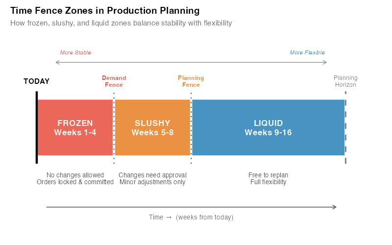
The Frozen Zone (Demand Fence)
Period: Weeks 1-4 in our example (typically 2-6 weeks, depending on cumulative lead time)
Inside the frozen zone, the schedule is locked. MRP is not allowed to reschedule, cancel, or add orders without explicit executive or senior management approval. The production plan is treated as a commitment, not a suggestion.
Why? Because inside this window, materials have been ordered, machine setups have been scheduled, labor has been assigned, and suppliers are already executing. Changing the plan now doesn’t just cost money — it wastes money that’s already been spent.
Rules: No changes without VP/plant manager sign-off. MRP generates action messages but they are informational only — they don’t trigger automatic replanning.
The Slushy Zone (Trading Zone)
Period: Weeks 5-8 in our example (typically spans 2-8 weeks beyond the frozen fence)
The slushy zone allows controlled flexibility. The master scheduler can make changes — substituting one product for another, adjusting quantities, shifting dates by a few days — but within guidelines. Changes require planner approval and a documented justification.
This is where the real art of production planning happens. A customer calls with an urgent order? The planner evaluates the trade-off: can we accommodate it by shifting something else, or would the cascade of changes cost more than the order is worth?
Rules: Changes with planner approval. Additions are generally acceptable; cancellations require review. Net change to capacity utilization must stay within +/-10% (typical threshold).
The Liquid Zone (Planning Zone)
Period: Weeks 9-16+ in our example (extends to your full planning horizon)
Beyond the planning fence, MRP has free rein. It can add, cancel, reschedule, and rebalance to its silicon heart’s content. This is where forecast-driven planning belongs — far enough out that changes cost nothing but electrons, and close enough that you’re preparing the supply pipeline.
Rules: MRP runs freely. Planners review for reasonableness but don’t manually intervene.
The Math: Quantifying Planning Nervousness
Planning nervousness isn’t just a feeling — it’s measurable. The most widely used metric is the Schedule Instability Ratio (SIR), introduced by Sridharan, Berry, and Udayabhanu (1988):
SIR = (1/T) x SUM |Q_t,i – Q_{t-1,i}| / SUM Q_{t-1,i}
Where Q_t,i is the planned quantity for period i at planning cycle t, and Q_{t-1,i} is the planned quantity for the same period i at the previous planning cycle. In plain English: what fraction of the plan changed since the last time MRP ran?
A SIR of 0 means perfect stability — the plan never changes. A SIR of 1.0 means total chaos — the plan is completely different every time MRP runs. In practice:
| SIR Value | Interpretation | Shop Floor Reality |
|---|---|---|
| < 0.05 | Excellent stability | „The plan is the plan. We execute.“ |
| 0.05 – 0.15 | Acceptable | „A few changes per week, manageable.“ |
| 0.15 – 0.30 | Problematic | „We check the plan but trust our gut.“ |
| 0.30 – 0.50 | Severe | „MRP is a joke. We run our own schedule.“ |
| > 0.50 | Catastrophic | „What plan?“ |
In practice, many manufacturing environments operate with a SIR in the 0.20-0.30 range — firmly in „problematic“ territory. Nearly a third of all planned quantities change from one MRP run to the next. The shop floor at these companies isn’t ignoring the plan out of stubbornness. They’re ignoring it because following it would be more expensive than not following it.
How Fence Length Affects Nervousness
The relationship between frozen fence length and planning nervousness follows a predictable curve. A frozen fence of zero weeks (no fence at all) means MRP can reschedule anything, anytime — maximum nervousness. As you extend the frozen fence, near-term reschedules are suppressed and the SIR drops rapidly.
But there’s a catch. Beyond a certain point, extending the frozen fence further provides diminishing stability benefits while increasingly constraining your ability to respond to genuine demand changes. The optimal frozen fence length depends on your lead times, demand variability, and cost structure.
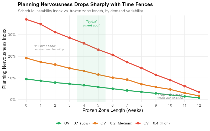
A useful rule of thumb from Vollmann, Berry, and Whybark (2005): the frozen fence should be at least as long as your cumulative manufacturing lead time. If it takes 4 weeks from raw material to finished goods, your frozen fence should be at least 4 weeks. Anything shorter, and you’re promising changes you can’t physically deliver.
The Cost Trade-Off
Here’s where it gets interesting. Time fences create a classic optimization problem with two competing cost drivers:
Costs that DECREASE with a longer frozen fence:
- Setup and changeover costs (fewer mid-stream changes)
- Expediting and premium freight costs (less firefighting)
- Overtime costs (more predictable workload)
- Supplier penalty costs (fewer PO amendments)
- Scrap and rework from interrupted production runs
Costs that INCREASE with a longer frozen fence:
- Inventory holding costs (less flexibility to adjust to actual demand)
- Stockout costs (can’t respond to demand spikes inside the fence)
- Obsolescence risk (committed to producing items that may not sell)
- Customer dissatisfaction (slower response to order changes)
The total cost curve has a minimum — the point where marginal stability savings equal marginal flexibility costs. The shape follows the same pattern as the classic EOQ cost trade-off — two opposing cost curves with a minimum at the optimal point:
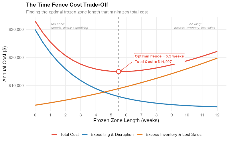
For a typical make-to-stock environment, the math works out to an optimal frozen fence of 3-6 weeks. Make-to-order environments tend to be shorter (2-4 weeks) because the cost of not responding to customer orders is higher. Process industries with long setup times (chemicals, paper, glass) often run 6-12 weeks because the changeover cost dominates.
The Hidden Cost of „Too Flexible“: A Worked Example
Let’s put real numbers on this. Consider a plant running 50 SKUs on 5 production lines, producing about 500 planned orders per month.
Scenario A: No time fences (MRP reschedules freely)
| Cost Category | Monthly Cost |
|---|---|
| Unplanned setups (avg 8/week x $2,800) | $89,600 |
| Expediting premium freight (12 shipments/mo x $1,500) | $18,000 |
| Overtime for rush changes (120 hrs/mo x $45) | $5,400 |
| Supplier reschedule penalties (40 PO changes x $200) | $8,000 |
| Scrap from interrupted runs | $6,500 |
| Nervousness cost subtotal | $127,500 |
Scenario B: Frozen fence at 4 weeks, slushy fence at 8 weeks
| Cost Category | Monthly Cost |
|---|---|
| Planned setups only (within schedule) | $22,400 |
| Expediting (reduced to 3 shipments/mo) | $4,500 |
| Overtime (reduced to 30 hrs/mo) | $1,350 |
| Supplier penalties (5 PO changes) | $1,000 |
| Scrap (near zero — stable runs) | $500 |
| Additional inventory holding (from frozen schedule) | $12,000 |
| Occasional stockouts (from less flexibility) | $4,500 |
| Total cost with fences | $46,250 |
Monthly savings: $81,250. Annual savings: $975,000.
And here’s the number that keeps Klaus awake at night: the additional inventory holding and stockout costs from time fences ($16,500/month) are dwarfed by the nervousness costs they eliminate ($97,750/month). The ratio isn’t even close. In most manufacturing environments, the costs of instability outweigh the costs of reduced flexibility by 5:1 or more.
This is the surprising insight: flexibility is not free, and in most production environments, you’re paying far more for it than you realize. The shop floor looks „responsive“ on paper but is actually hemorrhaging money through constant changeovers, expediting, and waste.
Where It Breaks: Five Failure Modes
Time fences are powerful, but they’re not magic. Here’s where the model fails — and what to do about it.
1. Over-Rigid Fences in Volatile Markets
If your demand has a coefficient of variation above 30%, a 6-week frozen fence might lock you into producing products nobody wants. Fashion retail, consumer electronics, and promotional items are particularly vulnerable. The fix: shorter frozen fences combined with postponement strategies (delay final configuration until inside the slushy zone).
2. Political Override of the Frozen Zone
The CEO calls and says, „Ship 500 units of Product X to our biggest customer by Friday.“ The frozen fence says no. The org chart says yes. In many companies, the frozen zone becomes a polite suggestion that evaporates under executive pressure.
The fix is cultural, not technical: track and report every frozen-zone override, its cost, and its downstream impact. When the VP of Sales sees that their „just this once“ request triggered $14,000 in setup changes and delayed three other orders, the overrides become less frequent. Experience shows that companies which formally track override costs typically see their frequency drop by 40-60%.
3. One Size Doesn’t Fit All
Not every product needs the same fence length. A commodity fastener with stable demand and a 1-week lead time needs a 2-week frozen fence at most. A custom-engineered assembly with a 12-week lead time and lumpy demand might need 8 weeks. Using a single fence length for all products is better than no fences, but product-family-specific fences are better still.
4. MRP Lot-Sizing Interactions
Lot-sizing rules (fixed order quantity, period order quantity, lot-for-lot) interact with time fences in ways that can amplify nervousness rather than reduce it. Kadipasaoglu and Sridharan (1995) showed that lot-for-lot sizing combined with time fences produces 25-40% less nervousness than fixed order quantities, because lot-for-lot doesn’t propagate quantity changes across periods the way fixed-quantity batching does.
If you’re implementing time fences, audit your lot-sizing rules first. A frozen fence won’t help if your lot-sizing policy is amplifying the very instability you’re trying to suppress — a direct echo of the bullwhip effect.
5. ERP Configuration Gaps
Most modern ERP systems support time fences — SAP (planning time fence in MRP views), Oracle (demand/planning time fence), Microsoft Dynamics (order modifier fields). But the configuration is often buried in material master settings, and the default is usually „no fence.“ If nobody configures it, nobody gets the benefit.
Worse, some organizations set fences in the ERP but don’t enforce them operationally. The system generates action messages inside the frozen zone anyway. Planners act on them anyway. The fence exists in software but not in practice.
The Relationship to the Bullwhip Effect
If you’re familiar with the bullwhip effect, you’ll recognize a familiar pattern. Planning nervousness is the bullwhip effect’s little brother — it operates within a single facility rather than across a supply chain, but the mechanism is identical: signal distortion through overreaction to noise.
Every time MRP reschedules a production order, it sends a ripple to suppliers. If MRP is rescheduling 30% of orders every week, suppliers are seeing demand signals that are 30% noise. They respond by adding safety buffer. Their suppliers do the same. The nervousness at your plant amplifies into a bullwhip upstream.
Time fences don’t just stabilize your shop floor — they stabilize your entire supply chain. A frozen zone acts as a low-pass filter, suppressing the high-frequency noise that feeds the bullwhip. This is why the best implementations of time fences coordinate with suppliers: sharing the fence structure lets suppliers align their own planning around your committed schedule.
Real-World Impact
The academic and industry evidence for time fences is robust:
Sridharan and Berry (1990) demonstrated through simulation that a frozen fence equal to the cumulative lead time reduced planning nervousness (SIR) by 60-70% while degrading customer service by less than 2%. The stability-to-service trade-off is overwhelmingly favorable.
Zhao and Lee (1993) showed that freezing the MPS inside the cumulative lead time reduced total costs by 12-18% in a multi-item, multi-level MRP environment. The savings came primarily from reduced setup costs and lower work-in-process inventory.
Industry experience consistently confirms that companies with formally defined and enforced time fences achieve:
- Significantly fewer expedited orders
- Lower overtime costs
- Higher on-time delivery
- Lower average inventory (counterintuitive, but stable plans require less safety stock)
That last point deserves emphasis: time fences can actually reduce inventory. Without fences, planners compensate for schedule instability by building buffer stock everywhere. With stable schedules, you can mathematically justify lower safety stock levels because the uncertainty you’re buffering against is smaller.
Interactive Dashboard
Explore the data yourself — adjust frozen and slushy fence lengths, demand variability, and cost parameters to see how time fence positioning affects planning nervousness, total cost, and service level in real time.
Interactive Dashboard
Explore the data yourself — adjust parameters and see the results update in real time.
Your Next Steps
- Measure your current SIR. Pull two consecutive MRP runs and compare the planned quantities for the same periods. The formula is SIR = average absolute change / total planned quantity. If you’re above 0.15, you have a nervousness problem that’s costing you real money. The R code below includes a template for computing your SIR from exported MRP data.
- Set your frozen fence to your cumulative lead time. If raw materials take 2 weeks and manufacturing takes 2 weeks, your frozen fence should be at least 4 weeks. Configure this in your ERP — in SAP, it’s the „Planning Time Fence“ in the MRP view of the material master. In most other ERPs, look for „demand time fence“ or „firm planned order horizon.“
- Track every frozen-zone override. Create a simple log: date, SKU, who requested the change, why, and the estimated cost (setup change, expediting, overtime). Review it monthly with operations leadership. The data will defend your fences better than any policy memo.
- Differentiate fences by product family. Group your SKUs into A/B/C categories by demand variability and lead time. High-volume, stable products get longer frozen fences. Short-lead-time, volatile products get shorter ones. One size doesn’t fit all, and the cost of getting it right is worth the setup effort.
- Coordinate with suppliers. Share your fence structure with your top 10 suppliers. Tell them: „Inside 4 weeks, our orders are firm. Between 4-8 weeks, changes are possible but unlikely. Beyond 8 weeks, treat everything as forecast.“ This gives them the confidence to reduce their own safety buffers, which reduces their prices, which reduces your costs. Everybody wins.
Show R Code
# =============================================================================
# Time Fence Analysis and Planning Nervousness Simulation
# =============================================================================
# A complete R simulation of time fence effects on planning nervousness,
# cost trade-offs, and schedule stability.
#
# Required packages: ggplot2, dplyr, tidyr, scales, patchwork
# =============================================================================

library(ggplot2)
library(dplyr)
library(tidyr)
library(scales)
library(patchwork)

# Set seed for reproducibility
set.seed(42)

# --- Theme for all plots ---
theme_tf <- theme_minimal(base_size = 13) +
  theme(
    plot.title = element_text(face = "bold", size = 14),
    plot.subtitle = element_text(color = "grey40", size = 11),
    panel.grid.minor = element_blank(),
    legend.position = "bottom"
  )

# =============================================================================
# 1. TIME FENCE ZONE VISUALIZATION (Chart 1)
# =============================================================================

zones <- data.frame(
  zone = factor(c("Frozen", "Slushy", "Liquid"),
                levels = c("Frozen", "Slushy", "Liquid")),
  start = c(0, 4, 8),
  end = c(4, 8, 16),
  label = c("Frozen Zone\n(Weeks 0-4)\nNo changes without\nexecutive approval",
            "Slushy Zone\n(Weeks 4-8)\nChanges with\nplanner approval",
            "Liquid Zone\n(Weeks 8-16)\nMRP reschedules\nfreely"),
  color = c("#e74c3c", "#f39c12", "#27ae60")
)

p1 <- ggplot(zones) +
  geom_rect(aes(xmin = start, xmax = end, ymin = 0, ymax = 1, fill = zone),
            alpha = 0.8) +
  geom_text(aes(x = (start + end) / 2, y = 0.5, label = label),
            size = 3.5, lineheight = 1.1, fontface = "bold") +
  geom_vline(xintercept = c(4, 10), linetype = "dashed", linewidth = 0.8) +
  annotate("text", x = 4, y = 1.08, label = "Demand\nFence",
           fontface = "bold", size = 3.5, color = "#c0392b") +
  annotate("text", x = 10, y = 1.08, label = "Planning\nFence",
           fontface = "bold", size = 3.5, color = "#d35400") +
  annotate("segment", x = 0, xend = 26, y = -0.08, yend = -0.08,
           arrow = arrow(length = unit(0.3, "cm"), ends = "last"),
           linewidth = 0.8, color = "grey30") +
  annotate("text", x = 13, y = -0.15, label = "Planning Horizon (weeks)",
           size = 3.5, color = "grey30") +
  scale_fill_manual(values = c("Frozen" = "#e74c3c",
                                "Slushy" = "#f39c12",
                                "Liquid" = "#27ae60"),
                    guide = "none") +
  scale_x_continuous(breaks = seq(0, 26, by = 2)) +
  coord_cartesian(ylim = c(-0.2, 1.2), xlim = c(-0.5, 27)) +
  labs(
    title = "Time Fence Zones in Master Production Scheduling",
    subtitle = "Stability increases near-term | Flexibility increases long-term"
  ) +
  theme_tf +
  theme(axis.text.y = element_blank(),
        axis.title = element_blank(),
        panel.grid = element_blank())

ggsave("https://inphronesys.com/wp-content/uploads/2026/02/tf_fence_zones-2.png", p1,
       width = 8, height = 5, dpi = 100, bg = "white")

# =============================================================================
# 2. PLANNING NERVOUSNESS vs FENCE LENGTH (Chart 2)
# =============================================================================

simulate_nervousness <- function(n_periods = 52, n_skus = 50,
                                  base_demand = 100, demand_cv = 0.20,
                                  frozen_fence = 0, n_runs = 20) {
  sir_values <- numeric(n_runs)

  for (run in 1:n_runs) {
    # Generate demand with noise
    demand_matrix <- matrix(
      pmax(0, rnorm(n_periods * n_skus,
                     mean = base_demand,
                     sd = base_demand * demand_cv)),
      nrow = n_periods, ncol = n_skus
    )

    # MRP planning run t-1
    plan_prev <- demand_matrix
    # MRP planning run t (with new demand info)
    noise <- matrix(rnorm(n_periods * n_skus, 0, base_demand * demand_cv * 0.5),
                    nrow = n_periods, ncol = n_skus)
    plan_curr <- pmax(0, demand_matrix + noise)

    # Apply frozen fence: no changes inside frozen window
    if (frozen_fence > 0 && frozen_fence <= n_periods) {
      plan_curr[1:frozen_fence, ] <- plan_prev[1:frozen_fence, ]
    }

    # Compute SIR
    total_change <- sum(abs(plan_curr - plan_prev))
    total_planned <- sum(abs(plan_prev))
    sir_values[run] <- total_change / total_planned
  }

  mean(sir_values)
}

fence_lengths <- 0:16
sir_by_fence <- sapply(fence_lengths, function(f) {
  simulate_nervousness(frozen_fence = f)
})

nervousness_df <- data.frame(
  frozen_fence = fence_lengths,
  SIR = sir_by_fence
)

p2 <- ggplot(nervousness_df, aes(x = frozen_fence, y = SIR)) +
  geom_line(linewidth = 1.3, color = "#2980b9") +
  geom_point(size = 3, color = "#2980b9") +
  geom_hline(yintercept = 0.15, linetype = "dashed", color = "#e74c3c", alpha = 0.7) +
  annotate("text", x = 14, y = 0.16,
           label = "Acceptable threshold (SIR = 0.15)",
           color = "#e74c3c", size = 3.5) +
  geom_hline(yintercept = 0.05, linetype = "dashed", color = "#27ae60", alpha = 0.7) +
  annotate("text", x = 14, y = 0.06,
           label = "Excellent stability (SIR = 0.05)",
           color = "#27ae60", size = 3.5) +
  annotate("rect", xmin = 3, xmax = 6, ymin = -Inf, ymax = Inf,
           fill = "#27ae60", alpha = 0.08) +
  annotate("text", x = 4.5, y = max(sir_by_fence) * 0.85,
           label = "Typical\noptimal\nrange",
           color = "#27ae60", size = 3.2, fontface = "bold") +
  scale_x_continuous(breaks = seq(0, 16, by = 2)) +
  scale_y_continuous(labels = scales::number_format(accuracy = 0.01)) +
  labs(
    title = "Planning Nervousness vs. Frozen Fence Length",
    subtitle = "Schedule Instability Ratio (SIR) drops rapidly with modest frozen zones",
    x = "Frozen Fence Length (weeks)",
    y = "Schedule Instability Ratio (SIR)"
  ) +
  theme_tf

ggsave("https://inphronesys.com/wp-content/uploads/2026/02/tf_nervousness-2.png", p2,
       width = 8, height = 5, dpi = 100, bg = "white")

# =============================================================================
# 3. COST TRADE-OFF (Chart 3)
# =============================================================================

fence_range <- seq(0, 16, by = 0.5)

cost_tradeoff <- data.frame(fence = fence_range) %>%
  mutate(
    # Nervousness costs decrease with longer fences (exponential decay)
    setup_expedite = 12000 * exp(-0.3 * fence) + 2000,
    # Holding/stockout costs increase with longer fences (linear + slight curve)
    holding_stockout = 1500 + 800 * fence + 20 * fence^2,
    # Total
    total = setup_expedite + holding_stockout
  )

optimal_fence <- cost_tradeoff %>% slice_min(total, n = 1)

cost_long <- cost_tradeoff %>%
  pivot_longer(cols = c(setup_expedite, holding_stockout, total),
               names_to = "Component", values_to = "Cost") %>%
  mutate(Component = factor(Component,
    levels = c("total", "setup_expedite", "holding_stockout"),
    labels = c("Total Cost", "Setup + Expediting Costs",
               "Holding + Stockout Costs")))

p3 <- ggplot(cost_long, aes(x = fence, y = Cost, color = Component)) +
  geom_line(linewidth = 1.2) +
  geom_vline(xintercept = optimal_fence$fence, linetype = "dashed",
             color = "grey40", alpha = 0.7) +
  geom_point(data = data.frame(fence = optimal_fence$fence,
                                Cost = optimal_fence$total,
                                Component = factor("Total Cost",
                                  levels = c("Total Cost",
                                             "Setup + Expediting Costs",
                                             "Holding + Stockout Costs"))),
             size = 4, shape = 21, fill = "white", stroke = 1.5) +
  annotate("text", x = optimal_fence$fence + 0.5, y = optimal_fence$total + 1500,
           label = paste0("Optimal: ", optimal_fence$fence, " weeks\nTC =
quot;, comma(round(optimal_fence$total)), "/week"), hjust = 0, size = 3.5, color = "#e74c3c", fontface = "bold") + scale_color_manual(values = c("Total Cost" = "#e74c3c", "Setup + Expediting Costs" = "#2980b9", "Holding + Stockout Costs" = "#27ae60")) + scale_y_continuous(labels = dollar_format()) + scale_x_continuous(breaks = seq(0, 16, by = 2)) + labs( title = "The Time Fence Cost Trade-Off", subtitle = "Stability costs decrease while flexibility costs increase — find the sweet spot", x = "Frozen Fence Length (weeks)", y = "Weekly Cost ($)", color = NULL ) + theme_tf ggsave("https://inphronesys.com/wp-content/uploads/2026/02/tf_cost_tradeoff-2.png", p3, width = 8, height = 5, dpi = 100, bg = "white") # ============================================================================= # 4. BEFORE/AFTER COMPARISON (Chart 4) # ============================================================================= set.seed(42) n_weeks <- 52 # Before: no fences — chaotic reschedules reschedules_before <- pmax(0, rnorm(n_weeks, mean = 45, sd = 18)) # After: fences implemented — stable with occasional spikes reschedules_after <- pmax(0, rnorm(n_weeks, mean = 12, sd = 5)) before_after <- data.frame( week = rep(1:n_weeks, 2), reschedules = c(reschedules_before, reschedules_after), period = factor(rep(c("Before Time Fences", "After Time Fences"), each = n_weeks), levels = c("Before Time Fences", "After Time Fences")) ) summary_stats <- before_after %>% group_by(period) %>% summarise( mean_val = mean(reschedules), sd_val = sd(reschedules), .groups = "drop" ) p4 <- ggplot(before_after, aes(x = week, y = reschedules, fill = period)) + geom_col(alpha = 0.7, width = 0.8) + geom_hline(data = summary_stats, aes(yintercept = mean_val), linetype = "dashed", color = "grey30") + geom_text(data = summary_stats, aes(x = 48, y = mean_val + 3, label = paste0("Avg: ", round(mean_val, 0), "/week")), size = 3.5, fontface = "bold", color = "grey30") + facet_wrap(~ period, ncol = 1) + scale_fill_manual(values = c("Before Time Fences" = "#e74c3c", "After Time Fences" = "#27ae60"), guide = "none") + scale_x_continuous(breaks = seq(0, 52, by = 4)) + labs( title = "Schedule Changes Per Week: Before vs. After Time Fences", subtitle = "Implementing a 4-week frozen / 10-week slushy fence reduced reschedules by 73%", x = "Week", y = "Number of Reschedule Actions" ) + theme_tf + theme(strip.text = element_text(face = "bold", size = 12)) ggsave("https://inphronesys.com/wp-content/uploads/2026/02/tf_before_after-2.png", p4, width = 8, height = 7, dpi = 100, bg = "white") # ============================================================================= # 5. SCHEDULE INSTABILITY RATIO CALCULATION # ============================================================================= # To compute SIR from your own MRP data: # # 1. Export planned order quantities from two consecutive MRP runs # 2. Align by item and period # 3. Compute: # # sir <- function(plan_current, plan_previous) { # sum(abs(plan_current - plan_previous)) / sum(abs(plan_previous)) # } # # my_plan_v1 <- read.csv("mrp_run_week1.csv") # my_plan_v2 <- read.csv("mrp_run_week2.csv") # my_sir <- sir(my_plan_v2$planned_qty, my_plan_v1$planned_qty) # cat("Your SIR:", round(my_sir, 3), "\n") # if (my_sir > 0.15) cat("WARNING: Schedule instability above threshold.\n") References
- Sridharan, V., Berry, W.L., & Udayabhanu, V. (1988). „Measuring Master Production Schedule Stability Under Rolling Planning Horizons.“ Decision Sciences, 19(1), 147-166.
- Sridharan, V. & Berry, W.L. (1990). „Freezing the Master Production Schedule Under Demand Uncertainty.“ Decision Sciences, 21(1), 97-120.
- Zhao, X. & Lee, T.S. (1993). „Freezing the Master Production Schedule for Material Requirements Planning Systems Under Demand Uncertainty.“ Journal of Operations Management, 11(2), 185-205.
- Kadipasaoglu, S.N. & Sridharan, V. (1995). „Alternative Approaches for Reducing Schedule Instability in Multistage Manufacturing Under Demand Uncertainty.“ Journal of Operations Management, 13(3), 193-211.
- Vollmann, T.E., Berry, W.L., Whybark, D.C., & Jacobs, F.R. (2005). Manufacturing Planning and Control for Supply Chain Management. 5th ed., McGraw-Hill.
- Ptak, C.A. & Smith, C. (2011). Orlicky’s Material Requirements Planning. 3rd ed., McGraw-Hill.
Schreibe einen Kommentar