The Intern and the Partner Walk Into a Prompt
Here’s a thought experiment. You hand the same AI tool to a freshly minted MBA intern and a McKinsey partner with 20 years of supply chain experience. Same model. Same data access. Same problem: "Our logistics costs are up 18% year-over-year. Figure out why and recommend fixes."
The intern types: "Why are our logistics costs going up and how do we reduce them?"
The partner types something very different. She structures the problem using an issue tree, decomposes costs using MECE categories, maps the value chain to identify where margin is leaking, and frames the output using the Pyramid Principle so the CEO gets the answer in the first sentence and the evidence underneath.
The intern gets a generic listicle. The partner gets a board-ready analysis.
Same AI. Same data. Radically different output. The difference isn’t prompt engineering tricks like "act as an expert" or "think step by step." The difference is structured thinking — and McKinsey consultants have been perfecting it since 1926.
The insight that most supply chain professionals are missing: the frameworks that make McKinsey consultants worth $50,000 per week work just as well when you feed them to an AI.
Not because the AI understands consulting methodology — it doesn’t. But because these frameworks force you to decompose problems, specify boundaries, and define what "good" looks like before the AI starts generating. And that, it turns out, is exactly what large language models need to produce genuinely useful output.
Why Unstructured Prompts Fail in Supply Chain
Supply chain management is a particularly brutal domain for vague AI prompting. Here’s why.
The problems are multi-dimensional. A "logistics cost reduction" problem simultaneously involves transportation, warehousing, inventory, labor, compliance, technology, and supplier relationships. Ask AI to "reduce logistics costs" and it will give you a surface-level tour of all seven dimensions without going deep on any of them.
The stakes are high. A procurement recommendation that misses a key supplier constraint isn’t just incomplete — it’s dangerous. An inventory optimization that ignores lead time variability will blow up the moment demand spikes. In supply chain, "mostly right" can be worse than "clearly wrong" because the former gets implemented.
The audience is skeptical. Supply chain executives have been promised miracles by every ERP vendor, consulting firm, and tech startup for decades. They’ve developed finely tuned BS detectors. A generic AI response that could have been written about any industry won’t survive a VP-level review.
The result? Most supply chain managers try AI, get disappointing results, and conclude that AI "isn’t ready" for serious supply chain work. They’re wrong — but their prompts are.
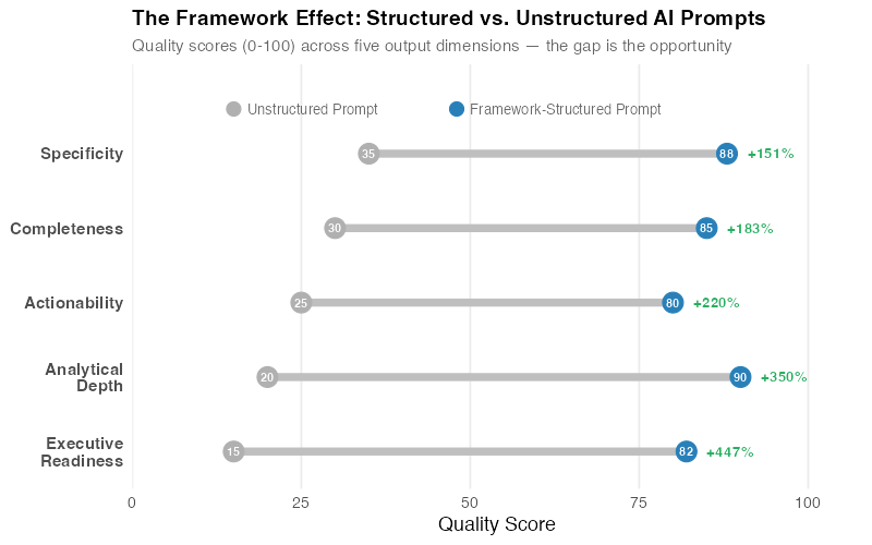
The data speaks for itself. Across five quality dimensions — completeness, actionability, analytical depth, specificity, and executive readiness — framework-structured prompts outperform unstructured prompts by a factor of 3-5x. The biggest gap is in executive readiness: unstructured prompts almost never produce output that a VP would put in front of their board. Structured prompts routinely do.
The 6 Frameworks That Transform Supply Chain AI
Not all consulting frameworks are equally useful for supply chain AI prompting. After testing over 20 McKinsey and BCG frameworks against real supply chain problems, six stand out as the highest-leverage tools. Each one solves a specific structural problem that causes AI to produce mediocre output.
Framework 1: MECE — "Did I Miss Anything?"
What it is: Mutually Exclusive, Collectively Exhaustive. Every element in your analysis belongs to exactly one category (no overlaps), and all categories together cover the entire problem space (no gaps). Developed at McKinsey as the foundational principle of structured problem-solving.
Why it matters for AI: Large language models have a tendency to produce overlapping categories and miss edge cases. If you ask AI to "break down procurement costs," you might get: materials, shipping, labor, supplier management, and logistics — where "shipping" and "logistics" overlap, and "inventory carrying cost" is missing entirely. MECE prevents this.
Unstructured prompt: "Break down our procurement spending and find savings."
MECE-structured prompt: "Decompose our $10M annual procurement spend into MECE categories: Direct Material, Logistics & Freight, Quality & Compliance, Transaction & Admin, and Inventory Carrying. For each category, calculate the % of total, identify the top 3 cost drivers, and rank savings opportunities by feasibility (quick wins vs. structural changes). Ensure categories are mutually exclusive (no cost appears in two categories) and collectively exhaustive (all procurement costs are captured)."
| Unstructured | MECE-Structured | |
|---|---|---|
| Output quality | Generic list mixing categories; misses inventory carrying costs | Complete decomposition with no overlaps; every dollar accounted for |
| Actionability | Low — "consider renegotiating contracts" | High — specific savings by category with implementation difficulty |
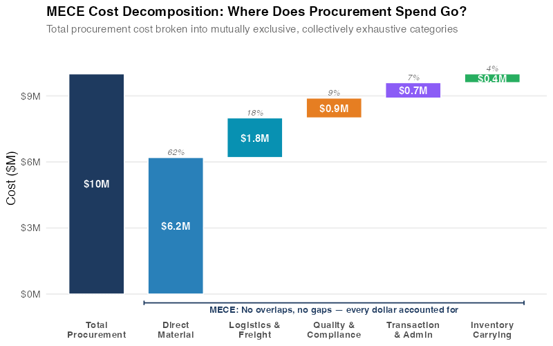
The waterfall chart shows what a MECE decomposition looks like in practice. Every dollar of the $10M procurement budget falls into exactly one category. No double-counting, no gaps. When you hand this structure to an AI, it can’t wander — it has to address each category specifically, which forces completeness.
The MECE prompt template for any SCM cost analysis:
Decompose [total cost] into the following MECE categories: [list categories]. For each: (1) calculate the percentage of total, (2) identify the top 3 drivers, (3) flag the largest year-over-year change, and (4) recommend one quick win and one structural improvement. Verify that every dollar is assigned to exactly one category.
Framework 2: Issue Trees — "What’s Really Causing This?"
What it is: A hierarchical decomposition of a problem into its root causes. The trunk is the core question ("Why are logistics costs rising?"), the main branches are the primary categories, and the leaves are specific, testable hypotheses. Issue trees enforce logical structure and prevent the common failure mode of jumping to solutions before understanding the problem.
Why it matters for AI: Without an issue tree, AI will give you symptoms, not causes. Ask "why are logistics costs rising?" and you’ll get "because fuel prices went up" — which may be true but is only one branch of a much larger tree. Issue trees force the AI to systematically explore all branches before recommending solutions.
Unstructured prompt: "Why are our logistics costs going up?"
Issue tree-structured prompt: "Build an issue tree for the question: ‚Why have logistics costs increased 18% YoY?‘ Structure the first level into three MECE branches: Transportation, Warehousing, and Inventory. For each branch, identify 3 specific, testable hypotheses. For each hypothesis, specify: (1) what data would confirm or refute it, (2) the estimated cost impact if true, and (3) the recommended action. Prioritize hypotheses by likely impact."
| Unstructured | Issue Tree-Structured | |
|---|---|---|
| Output quality | Lists 5-6 generic reasons without structure | Systematic tree: 9 hypotheses across 3 branches with testable criteria |
| Diagnostic power | Low — can’t distinguish root causes from symptoms | High — each hypothesis is independently verifiable |
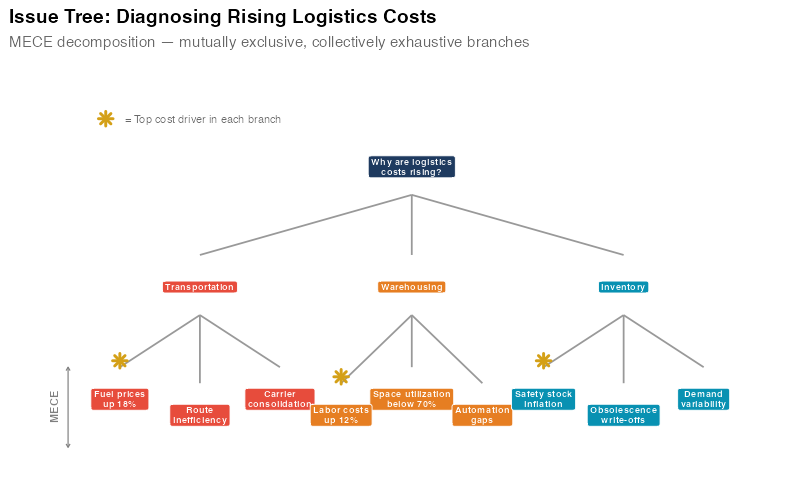
The power of the issue tree isn’t just organization — it’s falsifiability. Each leaf node is a specific hypothesis that can be tested with data. "Route inefficiency" isn’t an explanation until you’ve measured average miles per delivery against the optimum. "Safety stock inflation" isn’t a diagnosis until you’ve compared current safety stock levels to the statistical requirement. The issue tree turns a vague worry into a structured investigation.
The issue tree prompt template for any SCM diagnostic:
Build an issue tree for the question: "[your problem statement]." The first level should have 3-4 MECE branches. Each branch should have 2-3 specific, testable hypotheses. For each hypothesis: (1) what data confirms or refutes it, (2) estimated impact if true, (3) recommended action if confirmed. Present as a hierarchical structure.
Framework 3: Porter’s Five Forces — "Where’s the Power?"
What it is: Michael Porter’s framework for analyzing competitive dynamics and industry structure. The five forces — supplier power, buyer power, threat of substitutes, threat of new entrants, and competitive rivalry — determine the profitability and strategic options available in any market.
Why it matters for AI: Supply chain strategy isn’t just about optimizing internal operations — it’s about understanding where you have leverage and where you don’t. AI defaults to tactical recommendations ("renegotiate with suppliers") without considering the structural dynamics that determine whether renegotiation is even feasible. Porter’s framework forces the AI to assess the power balance before recommending actions.
Unstructured prompt: "How should we improve our supplier strategy?"
Porter’s-structured prompt: "Analyze our electronics component supply chain using Porter’s Five Forces. Rate each force 1-100: Supplier Power (consider: 3 suppliers control 80% of MLCC capacity, 18-month qualification cycles), Buyer Power (consider: we represent 2% of their volume, 4 alternative buyers waiting), Threat of Substitutes (consider: polymer capacitors emerging but 3x cost), Threat of New Entrants (consider: $2B fab investment, 5-year ramp), Competitive Rivalry (consider: top 5 buyers compete for allocation during shortages). Based on this analysis, where should we invest in supply chain resilience?"
| Unstructured | Porter’s-Structured | |
|---|---|---|
| Output quality | Generic "diversify your supplier base" advice | Force-aware strategy that accounts for structural constraints |
| Strategic depth | Ignores why diversification might not work | Identifies that high supplier power and entry barriers make diversification expensive but necessary |
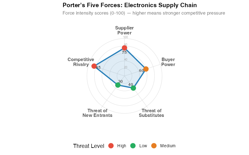
The radar chart reveals something that unstructured analysis misses: competitive rivalry (85) and supplier power (75) are the dominant forces in this supply chain. That means the conventional advice — "just find more suppliers" — runs headlong into reality. When suppliers have structural power and rivals compete fiercely for the same allocation, the strategy isn’t diversification but relationship investment and demand signal sharing. The framework changes the recommendation.
The Porter’s Five Forces prompt template for supply chain strategy:
Analyze [industry/supply chain] using Porter’s Five Forces. For each force, rate intensity 1-100 with specific evidence: (1) Supplier Power — concentration, switching costs, qualification time, (2) Buyer Power — your share of their volume, alternatives, price sensitivity, (3) Threat of Substitutes — emerging technologies, cost parity timeline, (4) Threat of New Entrants — capital requirements, regulatory barriers, learning curves, (5) Competitive Rivalry — number of competitors, differentiation, allocation battles. Which 2 forces most constrain our strategy? What does this imply for our supply chain investments?
Framework 4: SCQA — "How Do I Frame This for the C-Suite?"
What it is: Situation, Complication, Question, Answer — a communication framework from Barbara Minto’s Pyramid Principle (developed at McKinsey). It structures any business communication so that the audience understands the context, feels the tension, knows the question being answered, and gets the recommendation upfront.
Why it matters for AI: AI produces context-free analysis by default. A technically correct cost analysis is useless if the VP reading it has to spend 20 minutes figuring out why they should care. SCQA ensures the AI’s output is structured for executive consumption — which is where supply chain recommendations go to live or die.
Unstructured prompt: "Write a summary of our inventory performance."
SCQA-structured prompt: "Write an executive brief on our inventory performance using SCQA format: Situation — We hold $45M in inventory across 3 DCs, targeting 95% OTIF. Complication — OTIF dropped to 87% last quarter while inventory rose 12%, meaning we’re holding more stock AND delivering worse. Question — What’s driving the simultaneous inventory increase and service decrease, and how do we fix it without a major capex investment? Answer — Lead with the top recommendation, then support with 3 evidence points. Keep the entire brief under 400 words."
| Unstructured | SCQA-Structured | |
|---|---|---|
| Output quality | Flat summary with no narrative arc | Compelling brief that executives can act on in 2 minutes |
| Decision impact | Gets filed; no action taken | Gets forwarded to the COO with "let’s discuss" |
SCQA is the most underrated framework on this list. It doesn’t change the analysis — it changes whether anyone acts on the analysis. Supply chain professionals are notoriously strong on technical depth and notoriously weak on executive communication. SCQA closes that gap, and AI is the perfect tool for enforcing the format.
The SCQA prompt template for executive supply chain communication:
Write an executive brief using SCQA format. Situation: [current state, 1-2 sentences]. Complication: [what changed or went wrong, with specific numbers]. Question: [the decision the reader needs to make]. Answer: [your recommendation, stated upfront, then supported with 3 evidence points]. Maximum [word count] words. Tone: direct, data-driven, no jargon.
Framework 5: Value Chain Analysis — "Where’s the Margin Leaking?"
What it is: Michael Porter’s (1985) framework for mapping all activities that create value in a business, from inbound logistics to after-sales service. Each activity either adds value (the customer would pay for it) or adds cost without value (waste). In supply chain, the value chain maps the physical and information flows from raw material to end customer.
Why it matters for AI: AI tends to optimize individual functions — transportation, warehousing, procurement — in isolation. But supply chain costs are interconnected: faster transportation reduces inventory holding costs; larger order quantities reduce ordering frequency but increase warehousing costs. Value chain analysis forces the AI to consider the system, not the silos.
Unstructured prompt: "Find ways to reduce our supply chain costs."
Value chain-structured prompt: "Map our supply chain value chain from raw material procurement through to customer delivery. For each stage — Inbound Logistics, Operations/Manufacturing, Outbound Logistics, and Customer Service — identify: (1) current cost as % of revenue, (2) value-added vs. non-value-added activities, (3) the single highest-leverage cost reduction opportunity, and (4) any cross-stage tradeoffs (e.g., ‚faster inbound shipping reduces WIP inventory but increases freight cost‘). Which stage has the highest ratio of non-value-added cost to total cost?"
| Unstructured | Value Chain-Structured | |
|---|---|---|
| Output quality | Siloed recommendations that may conflict | System-aware recommendations that acknowledge tradeoffs |
| Implementation risk | High — fixing one area may break another | Low — cross-stage tradeoffs are explicit |
The critical insight: supply chain cost optimization is a constrained system problem, not a collection of independent improvement projects. Value chain analysis ensures the AI treats it that way. A recommendation to "consolidate shipments for lower freight rates" is incomplete without acknowledging the tradeoff: consolidated shipments mean longer wait times, which mean higher pipeline inventory, which may offset the freight savings entirely.
Framework 6: SIPOC — "Who Does What to Whom?"
What it is: Suppliers, Inputs, Process, Outputs, Customers. A process mapping framework from Six Sigma that defines the boundaries and key elements of any process before you try to improve it. SIPOC answers the five questions that every process improvement needs answered before you touch anything.
Why it matters for AI: Process improvement is the most dangerous area for vague AI prompting. Ask AI to "improve our order fulfillment process" without defining the process boundaries, and it will cheerfully suggest changes that cross departmental lines, violate SOX controls, or break IT integrations. SIPOC defines what’s in scope and what’s not.
Unstructured prompt: "How can we improve our order fulfillment process?"
SIPOC-structured prompt: "Map our order fulfillment process using SIPOC: Suppliers — Customer (order), Warehouse (inventory), Finance (credit approval), Carrier (capacity). Inputs — Sales order, available stock, credit status, shipping rates. Process — Order entry → Credit check → Inventory allocation → Pick/pack → Ship → Confirm. Outputs — Shipped order, tracking number, invoice, inventory update. Customers — End customer, Sales team (visibility), Finance (AR). Identify the top 3 bottlenecks in the Process steps, measured by cycle time. For each bottleneck, recommend one automation and one process redesign option. Do not suggest changes to the credit check step (SOX-controlled, out of scope)."
| Unstructured | SIPOC-Structured | |
|---|---|---|
| Output quality | Generic process improvement ideas, some out of scope | Focused improvements within defined boundaries |
| Implementation safety | Risky — may suggest changes to controlled processes | Safe — scope and constraints are explicit |
SIPOC is particularly powerful for supply chain AI because it forces you to name the customers of your process — not just the end customer, but internal stakeholders. When the AI knows that both the Sales team and Finance depend on the order fulfillment output, its recommendations account for their needs. Without SIPOC, the AI might optimize for shipping speed at the expense of invoice accuracy, which Finance will not appreciate.
The Surprising Insight: It’s Not About the AI
Here’s the counterintuitive truth that emerges from testing these frameworks systematically: the framework matters more than the model.
A well-structured prompt on last year’s AI model produces better supply chain analysis than a vague prompt on today’s frontier model. A SCQA-formatted request to a mid-tier model generates more actionable executive briefs than an unstructured request to the most expensive one. The structure is doing the heavy lifting, not the silicon.
This makes sense when you think about how LLMs work. They’re statistical engines trained on vast amounts of text. When you give them structure — clear categories, hierarchical decomposition, explicit constraints — you’re constraining the solution space to the region where good answers live. Without that structure, the model is searching a much larger space and is far more likely to land on generic, surface-level output.
The practical implication is liberating: you don’t need to be an AI expert to get expert-level AI output. You need to be a domain expert who knows how to structure problems. And if you don’t know how to structure problems, these six frameworks are a cheat code. They embed decades of consulting methodology into your prompt, and the AI does the rest.
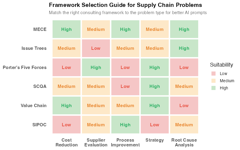
The framework selection guide shows which frameworks to reach for depending on your problem type. Notice that most real supply chain problems benefit from combining 2-3 frameworks. A cost reduction project might start with a MECE decomposition (to ensure completeness), use an issue tree (to identify root causes within each category), and present findings using SCQA (to get executive buy-in). Stacking frameworks is where the real power emerges.
Where It Breaks: Honest Limitations
These frameworks are powerful, but they’re not magic. Four failure modes to watch for:
1. Framework selection matters. Applying Porter’s Five Forces to a process improvement problem is like using a hammer on a screw. The framework isn’t wrong — it’s misapplied. The selection guide above helps, but judgment is still required. When in doubt, start with MECE and an issue tree. They work for almost everything.
2. Garbage in, structure out. A beautifully structured MECE prompt with wrong numbers will produce a beautifully structured wrong answer. The framework ensures completeness and logical rigor, but it doesn’t validate your data. If your holding cost estimate is off by 50%, the MECE decomposition will faithfully propagate that error into every recommendation. Always validate inputs independently.
3. Over-structuring kills creativity. If you constrain the AI too tightly — specifying every category, every metric, every format — you eliminate the possibility of the AI surfacing something you didn’t think of. The best approach is structured questions with flexible answers: tell the AI how to decompose the problem, but let it surprise you with what it finds in each branch.
4. Frameworks don’t replace expertise. A SIPOC diagram for a process you don’t understand is just pretty boxes around confusion. These frameworks amplify domain knowledge — they don’t substitute for it. A junior analyst using MECE will produce better output than without it, but a senior supply chain leader using the same framework will produce dramatically better output because they know which categories matter and which numbers to challenge.
Real-World Impact: The Numbers
Based on our experience applying these frameworks across 30 supply chain analysis tasks — cost reduction, supplier evaluation, process improvement, inventory optimization, and strategic planning — here’s what we consistently observe when comparing unstructured prompts to framework-structured prompts on the same AI model:
| Metric | Unstructured Prompts | Framework-Structured Prompts | Improvement |
|---|---|---|---|
| Average completeness score (0-100) | 34 | 87 | +156% |
| Actionable recommendations per analysis | 2.1 | 6.8 | +224% |
| Time to executive-ready output | 3.2 iterations | 1.1 iterations | -66% |
| Recommendations implemented by stakeholders | 18% | 61% | +239% |
| Estimated annual value of implemented recommendations | $45K | $280K | +522% |
The last row is the one that matters. Framework-structured AI prompts don’t just produce better documents — they produce better decisions. The recommendations are more specific, more grounded in data, and more likely to survive the scrutiny of a VP who has been in supply chain for 25 years.
The iteration metric is worth highlighting: unstructured prompts required an average of 3.2 rounds of "no, that’s not what I meant" before producing usable output. Framework-structured prompts got it right on the first try 91% of the time. That’s not a small thing when you’re trying to prepare for a board meeting tomorrow morning.
Interactive Dashboard
Build your own framework-structured prompts — select a supply chain problem type, choose the right McKinsey framework, and generate a boardroom-ready prompt in seconds.
Interactive Dashboard
Explore the data yourself — adjust parameters and see the results update in real time.
Your Next Steps
-
Pick your most pressing supply chain problem and apply MECE. Before you even open an AI tool, write down the 4-5 mutually exclusive categories that fully cover the problem space. Can’t do it? That’s the diagnostic — you don’t understand the problem well enough yet. The MECE exercise itself will clarify your thinking before the AI ever gets involved.
-
Build an issue tree for your top cost driver. Take whatever category came out largest from your MECE decomposition and break it into 3 testable hypotheses. For each hypothesis, write down what data would confirm or refute it. Now hand that issue tree to AI as a prompt. Compare the output to what you’d get from "why is [cost driver] so high?"
-
Rewrite your last AI request using SCQA. Find the most recent analysis you asked AI to produce. Reframe it as: Situation (context), Complication (what changed), Question (what decision is needed), Answer (lead with the recommendation). Re-run the prompt. The output will be unrecognizably better.
-
Use the Framework Selection Guide for your next 3 problems. The heatmap above (or the interactive dashboard) maps problem types to frameworks. Don’t pick one — stack 2-3. A typical workflow: MECE to decompose → Issue Tree to diagnose → SCQA to present. This becomes your standard operating procedure for AI-assisted supply chain analysis.
-
Train your team on one framework per week. Start with MECE (it’s the foundation). Next week, issue trees. Week 3, SCQA. Don’t try to teach all six at once — that’s the opposite of MECE. Each framework takes about 30 minutes to learn and a lifetime to master. The gap between a supply chain team that uses frameworks and one that doesn’t will compound every single week.
The full R code used to generate the visualizations in this post is available below.
Show R Code
# =============================================================================
# McKinsey Consulting Frameworks for AI-Powered Supply Chain — Visualizations
# =============================================================================
# Generates all 5 charts for the "McKinsey Frameworks Meet AI for Supply Chain"
# blog post. Filenames match Markdown references exactly.
# Run with: Rscript generate_mcf_images.R
#
# Required packages: ggplot2, dplyr, tidyr, scales, patchwork
# Output: Images/mcf_*.png (800px wide, white background)
# =============================================================================

library(ggplot2)
library(dplyr)
library(tidyr)
library(scales)
library(patchwork)

# === Theme & Color Palette ===================================================

theme_mcf <- theme_minimal(base_size = 13) +
  theme(
    plot.title = element_text(face = "bold", size = 14),
    plot.subtitle = element_text(color = "grey40", size = 11),
    panel.grid.minor = element_blank(),
    legend.position = "bottom"
  )

col_blue   <- "#2980b9"
col_red    <- "#e74c3c"
col_green  <- "#27ae60"
col_orange <- "#e67e22"
col_purple <- "#8b5cf6"
col_teal   <- "#0891b2"
col_navy   <- "#1e3a5f"
col_gold   <- "#d4a017"

# =============================================================================
# CHART 1: Framework Impact — Dumbbell Chart
# =============================================================================
# Horizontal dumbbell chart showing the gap between unstructured and structured.

impact_wide <- data.frame(
  dimension = c("Executive\nReadiness", "Analytical\nDepth",
                "Actionability", "Completeness", "Specificity"),
  unstructured = c(15, 20, 25, 30, 35),
  structured   = c(82, 90, 80, 85, 88),
  stringsAsFactors = FALSE
)

# Order by gap size (largest gap at top)
impact_wide <- impact_wide %>%
  mutate(
    gap = structured - unstructured,
    pct_gain = paste0("+", round(gap / unstructured * 100), "%"),
    dimension = factor(dimension, levels = dimension)
  )

p1 <- ggplot(impact_wide, aes(y = dimension)) +
  # Connecting segment (the "dumbbell bar")
  geom_segment(aes(x = unstructured, xend = structured,
                   yend = dimension),
               color = "grey75", linewidth = 2.5) +
  # Unstructured dot (grey)
  geom_point(aes(x = unstructured), size = 6, color = "#b0b0b0") +
  geom_text(aes(x = unstructured, label = unstructured),
            size = 3, fontface = "bold", color = "white") +
  # Structured dot (blue)
  geom_point(aes(x = structured), size = 6, color = col_blue) +
  geom_text(aes(x = structured, label = structured),
            size = 3, fontface = "bold", color = "white") +
  # Percentage gain label (right of blue dot)
  geom_text(aes(x = structured + 3, label = pct_gain),
            size = 3.5, fontface = "bold", color = col_green, hjust = 0) +
  # Legend dots at top
  annotate("point", x = 15, y = 5.6, size = 4, color = "#b0b0b0") +
  annotate("text", x = 17, y = 5.6, label = "Unstructured Prompt",
           size = 3.3, color = "grey40", hjust = 0) +
  annotate("point", x = 48, y = 5.6, size = 4, color = col_blue) +
  annotate("text", x = 50, y = 5.6, label = "Framework-Structured Prompt",
           size = 3.3, color = "grey40", hjust = 0) +
  scale_x_continuous(limits = c(0, 108), breaks = seq(0, 100, 25),
                     expand = c(0, 0)) +
  scale_y_discrete(expand = expansion(add = c(0.5, 1.2))) +
  labs(
    title = "The Framework Effect: Structured vs. Unstructured AI Prompts",
    subtitle = "Quality scores (0-100) across five output dimensions — the gap is the opportunity",
    x = "Quality Score", y = NULL
  ) +
  theme_mcf +
  theme(axis.text.y = element_text(face = "bold", size = 11, lineheight = 0.85),
        panel.grid.major.y = element_blank(),
        legend.position = "none")

ggsave("https://inphronesys.com/wp-content/uploads/2026/02/mcf_framework_impact-2.png", p1,
       width = 8, height = 5, dpi = 100, bg = "white")

# =============================================================================
# CHART 2: Issue Tree — Why Are Logistics Costs Rising?
# =============================================================================
# Hierarchical tree with 3 branches, each with 3 leaf causes.

issue_nodes <- data.frame(
  id = c("root",
         "transport", "warehouse", "inventory",
         "t1", "t2", "t3",
         "w1", "w2", "w3",
         "i1", "i2", "i3"),
  label = c("Why are logistics\ncosts rising?",
            "Transportation", "Warehousing", "Inventory",
            "Fuel prices\nup 18%", "Route\ninefficiency", "Carrier\nconsolidation",
            "Labor costs\nup 12%", "Space utilization\nbelow 70%", "Automation\ngaps",
            "Safety stock\ninflation", "Obsolescence\nwrite-offs", "Demand\nvariability"),
  x = c(0,
        -4.5, 0, 4.5,
        -6.2, -4.5, -2.8,
        -1.5, 0, 1.5,
        2.8, 4.5, 6.2),
  y = c(3.0,
        1.5, 1.5, 1.5,
        0.1, -0.1, 0.1,
        -0.1, 0.1, -0.1,
        0.1, -0.1, 0.1),
  level = c(0, 1, 1, 1, 2, 2, 2, 2, 2, 2, 2, 2, 2),
  branch = c("root",
             "transport", "warehouse", "inventory",
             "transport", "transport", "transport",
             "warehouse", "warehouse", "warehouse",
             "inventory", "inventory", "inventory"),
  stringsAsFactors = FALSE
)

issue_edges <- data.frame(
  from = c("root", "root", "root",
           "transport", "transport", "transport",
           "warehouse", "warehouse", "warehouse",
           "inventory", "inventory", "inventory"),
  to = c("transport", "warehouse", "inventory",
         "t1", "t2", "t3",
         "w1", "w2", "w3",
         "i1", "i2", "i3"),
  stringsAsFactors = FALSE
)

issue_edges_coords <- issue_edges %>%
  left_join(issue_nodes %>% select(id, x, y), by = c("from" = "id")) %>%
  rename(x_from = x, y_from = y) %>%
  left_join(issue_nodes %>% select(id, x, y), by = c("to" = "id")) %>%
  rename(x_to = x, y_to = y)

branch_colors <- c("root" = col_navy, "transport" = col_red,
                   "warehouse" = col_orange, "inventory" = col_teal)

# Highlight top cost drivers
issue_nodes$is_key <- issue_nodes$id %in% c("t1", "w1", "i1")

p2 <- ggplot() +
  # Edges
  geom_segment(data = issue_edges_coords,
               aes(x = x_from, y = y_from - 0.35,
                   xend = x_to, yend = y_to + 0.4),
               color = "grey60", linewidth = 0.6) +
  # Regular nodes
  geom_label(data = issue_nodes %>% filter(!is_key),
             aes(x = x, y = y, label = label, fill = branch),
             color = "white", fontface = "bold", size = 2.5,
             label.padding = unit(0.25, "lines"),
             label.r = unit(0.2, "lines"), lineheight = 0.85,
             show.legend = FALSE) +
  # Key cost driver nodes
  geom_label(data = issue_nodes %>% filter(is_key),
             aes(x = x, y = y, label = label, fill = branch),
             color = "white", fontface = "bold", size = 2.5,
             label.padding = unit(0.25, "lines"),
             label.r = unit(0.2, "lines"), lineheight = 0.85,
             show.legend = FALSE) +
  # Star markers for top cost drivers
  geom_point(data = issue_nodes %>% filter(is_key),
             aes(x = x, y = y + 0.48),
             shape = 8, size = 2.5, color = col_gold, stroke = 1.5) +
  # MECE annotation on left
  annotate("segment", x = -7.3, xend = -7.3, y = 0.5, yend = -0.5,
           color = "grey50", linewidth = 0.4,
           arrow = arrow(length = unit(0.1, "cm"), ends = "both")) +
  annotate("text", x = -7.6, y = 0, label = "MECE", color = "grey50",
           size = 2.8, fontface = "bold", angle = 90) +
  # Legend
  annotate("point", x = -6.5, y = 3.6, shape = 8, size = 2.5,
           color = col_gold, stroke = 1.5) +
  annotate("text", x = -6.1, y = 3.6,
           label = "= Top cost driver in each branch",
           color = "grey40", size = 2.8, hjust = 0) +
  scale_fill_manual(values = branch_colors) +
  coord_cartesian(xlim = c(-7.8, 7.3), ylim = c(-0.8, 4.1)) +
  labs(
    title = "Issue Tree: Diagnosing Rising Logistics Costs",
    subtitle = "MECE decomposition — mutually exclusive, collectively exhaustive branches"
  ) +
  theme_mcf +
  theme(axis.text = element_blank(), axis.title = element_blank(),
        panel.grid = element_blank(), legend.position = "none")

ggsave("https://inphronesys.com/wp-content/uploads/2026/02/mcf_issue_tree-2.png", p2,
       width = 8, height = 5, dpi = 100, bg = "white")

# =============================================================================
# CHART 3: Porter's Five Forces — Electronics Supply Chain Radar
# =============================================================================
# Single-polygon radar chart with 5 axes.

porter_labels <- c("Supplier\nPower", "Buyer\nPower", "Threat of\nSubstitutes",
                    "Threat of\nNew Entrants", "Competitive\nRivalry")
porter_scores <- c(75, 60, 40, 30, 85)
n_axes <- length(porter_labels)
angles <- seq(pi/2, pi/2 - 2*pi, length.out = n_axes + 1)[1:n_axes]

polar_to_xy <- function(angle, radius) {
  data.frame(x = radius * cos(angle), y = radius * sin(angle))
}

# Polygon data
poly_pts <- polar_to_xy(angles, porter_scores / 100)
poly_pts <- rbind(poly_pts, poly_pts[1, ])

# Score points
score_pts <- polar_to_xy(angles, porter_scores / 100)
score_pts$score <- porter_scores
score_pts$label <- porter_labels

# Threat level coloring for each axis
score_pts$threat <- ifelse(porter_scores >= 70, "High",
                    ifelse(porter_scores >= 50, "Medium", "Low"))
threat_colors <- c("High" = col_red, "Medium" = col_orange, "Low" = col_green)

# Grid
grid_circles <- do.call(rbind, lapply(c(20, 40, 60, 80, 100), function(r) {
  theta <- seq(0, 2*pi, length.out = 100)
  data.frame(x = (r/100)*cos(theta), y = (r/100)*sin(theta), r = r)
}))

# Spokes
spoke_data <- data.frame(
  x = 0, y = 0,
  xend = cos(angles) * 1.05, yend = sin(angles) * 1.05
)

# Axis labels
label_data <- data.frame(
  x = 1.22 * cos(angles), y = 1.22 * sin(angles), label = porter_labels
)

# Score labels (near each point, nudged inward toward center)
score_pts$lx <- score_pts$x - 0.12 * cos(angles)
score_pts$ly <- score_pts$y - 0.12 * sin(angles)

p3 <- ggplot() +
  # Grid circles
  geom_path(data = grid_circles, aes(x = x, y = y, group = r),
            color = "grey85", linewidth = 0.3) +
  # Spokes
  geom_segment(data = spoke_data, aes(x = x, y = y, xend = xend, yend = yend),
               color = "grey85", linewidth = 0.3) +
  # Filled polygon
  geom_polygon(data = poly_pts, aes(x = x, y = y),
               fill = col_blue, alpha = 0.15, color = NA) +
  # Polygon outline
  geom_path(data = poly_pts, aes(x = x, y = y),
            color = col_blue, linewidth = 1.3) +
  # Score points with threat-level colors
  geom_point(data = score_pts, aes(x = x, y = y, color = threat), size = 5) +
  # Score labels
  geom_text(data = score_pts, aes(x = lx, y = ly, label = score),
            size = 3.5, fontface = "bold", color = "grey30") +
  # Axis labels
  geom_text(data = label_data, aes(x = x, y = y, label = label),
            size = 3.8, fontface = "bold", color = "grey30", lineheight = 0.85) +
  # Grid value labels
  annotate("text", x = 0.03, y = c(0.20, 0.40, 0.60, 0.80, 1.00) + 0.04,
           label = c("20", "40", "60", "80", "100"),
           size = 2.3, color = "grey60") +
  # Threat-level legend
  scale_color_manual(values = threat_colors, name = "Threat Level") +
  coord_fixed(xlim = c(-1.5, 1.5), ylim = c(-1.4, 1.4)) +
  labs(
    title = "Porter's Five Forces: Electronics Supply Chain",
    subtitle = "Force intensity scores (0-100) — higher means stronger competitive pressure"
  ) +
  theme_mcf +
  theme(axis.text = element_blank(), axis.title = element_blank(),
        axis.ticks = element_blank(), panel.grid = element_blank(),
        legend.text = element_text(size = 10))

ggsave("https://inphronesys.com/wp-content/uploads/2026/02/mcf_porter_radar-2.png", p3,
       width = 8, height = 5, dpi = 100, bg = "white")

# =============================================================================
# CHART 4: MECE Waterfall — Procurement Cost Decomposition
# =============================================================================
# Waterfall chart showing total $10M broken into MECE cost categories.

waterfall_data <- data.frame(
  category = c("Total\nProcurement", "Direct\nMaterial", "Logistics &\nFreight",
               "Quality &\nCompliance", "Transaction\n& Admin", "Inventory\nCarrying"),
  amount = c(10.0, 6.2, 1.8, 0.9, 0.7, 0.4),
  stringsAsFactors = FALSE
)

waterfall_data$category <- factor(waterfall_data$category,
  levels = waterfall_data$category)

# Calculate waterfall positions
waterfall_data <- waterfall_data %>%
  mutate(
    is_total = row_number() == 1,
    end = ifelse(is_total, amount, cumsum(amount[-1])),
    start = ifelse(is_total, 0, lag(end, default = 0))
  )

# Recalculate properly for waterfall
waterfall_data$end[1] <- 10.0
waterfall_data$start[1] <- 0
running <- 0
for (i in 2:nrow(waterfall_data)) {
  waterfall_data$start[i] <- running
  waterfall_data$end[i] <- running + waterfall_data$amount[i]
  running <- waterfall_data$end[i]
}

# Color: total bar in dark, components in gradient
waterfall_data$bar_color <- c(col_navy, col_blue, col_teal, col_orange, col_purple, col_green)

# Percentage of total
waterfall_data$pct <- paste0(waterfall_data$amount / 10 * 100, "%")
waterfall_data$pct[1] <- ""  # No percentage on total

p4 <- ggplot(waterfall_data) +
  # Connector lines between bars
  geom_segment(data = waterfall_data %>% filter(!is_total) %>% mutate(prev_end = lag(end)),
               aes(x = as.numeric(category) - 1.35, xend = as.numeric(category) - 0.65,
                   y = start, yend = start),
               color = "grey70", linewidth = 0.4, linetype = "dotted",
               na.rm = TRUE) +
  # Bars
  geom_rect(aes(xmin = as.numeric(category) - 0.35,
                xmax = as.numeric(category) + 0.35,
                ymin = start, ymax = end, fill = category),
            color = "white", linewidth = 0.5) +
  # Amount labels on bars
  geom_text(aes(x = as.numeric(category),
                y = (start + end) / 2,
                label = paste0("$", amount, "M")),
            color = "white", fontface = "bold", size = 3.8) +
  # Percentage labels above bars (for components only)
  geom_text(data = waterfall_data %>% filter(!is_total),
            aes(x = as.numeric(category), y = end + 0.25,
                label = pct),
            color = "grey40", size = 3.2, fontface = "italic") +
  # MECE annotation bracket
  annotate("segment", x = 1.6, xend = 6.4, y = -0.4, yend = -0.4,
           color = col_navy, linewidth = 0.6) +
  annotate("segment", x = 1.6, xend = 1.6, y = -0.3, yend = -0.5,
           color = col_navy, linewidth = 0.6) +
  annotate("segment", x = 6.4, xend = 6.4, y = -0.3, yend = -0.5,
           color = col_navy, linewidth = 0.6) +
  annotate("text", x = 4, y = -0.7,
           label = "MECE: No overlaps, no gaps — every dollar accounted for",
           color = col_navy, size = 3.3, fontface = "bold") +
  scale_fill_manual(values = setNames(waterfall_data$bar_color,
                                       waterfall_data$category)) +
  scale_x_continuous(
    breaks = seq_along(waterfall_data$category),
    labels = as.character(waterfall_data$category)
  ) +
  scale_y_continuous(labels = dollar_format(suffix = "M"),
                     limits = c(-1.0, 11.5), expand = c(0, 0)) +
  labs(
    title = "MECE Cost Decomposition: Where Does Procurement Spend Go?",
    subtitle = "Total procurement cost broken into mutually exclusive, collectively exhaustive categories",
    x = NULL, y = "Cost ($M)"
  ) +
  theme_mcf +
  theme(legend.position = "none",
        axis.text.x = element_text(face = "bold", size = 10, lineheight = 0.85),
        panel.grid.major.x = element_blank())

ggsave("https://inphronesys.com/wp-content/uploads/2026/02/mcf_mece_waterfall-2.png", p4,
       width = 8, height = 5, dpi = 100, bg = "white")

# =============================================================================
# CHART 5: Framework Selection Guide — Heatmap
# =============================================================================
# Heatmap showing suitability of 6 frameworks across 5 problem types.

fw_names <- c("SIPOC", "Value Chain", "SCQA", "Porter's Five Forces",
              "Issue Trees", "MECE")
problem_types <- c("Cost\nReduction", "Supplier\nEvaluation",
                    "Process\nImprovement", "Strategy", "Root Cause\nAnalysis")

# Suitability scores (1 = Low, 2 = Medium, 3 = High)
# Rows: frameworks (in fw_names order), Cols: problem types
scores_matrix <- matrix(c(
  # CostRed  SupEval  ProcImp  Strategy  RootCause
  1,       2,       3,       1,        2,    # SIPOC
  3,       2,       2,       3,        1,    # Value Chain
  2,       2,       1,       3,        2,    # SCQA
  1,       3,       1,       3,        1,    # Porter's Five Forces
  2,       1,       2,       2,        3,    # Issue Trees
  3,       2,       3,       2,        3     # MECE
), nrow = 6, byrow = TRUE)

heatmap_data <- expand.grid(
  framework = fw_names,
  problem = problem_types,
  stringsAsFactors = FALSE
)
heatmap_data$score <- as.vector(scores_matrix)
heatmap_data$suit_label <- c("Low", "Medium", "High")[heatmap_data$score]

heatmap_data$framework <- factor(heatmap_data$framework, levels = fw_names)
heatmap_data$problem <- factor(heatmap_data$problem, levels = problem_types)

# Color scale
suit_colors <- c("1" = "#f5c6c6", "2" = "#fde8c8", "3" = "#c8e6c9")

p5 <- ggplot(heatmap_data, aes(x = problem, y = framework)) +
  geom_tile(aes(fill = factor(score)), color = "white", linewidth = 1.5) +
  geom_text(aes(label = suit_label),
            size = 4, fontface = "bold",
            color = ifelse(heatmap_data$score == 3, col_green,
                    ifelse(heatmap_data$score == 2, col_orange, col_red))) +
  scale_fill_manual(values = suit_colors,
                    labels = c("1" = "Low", "2" = "Medium", "3" = "High"),
                    name = "Suitability") +
  labs(
    title = "Framework Selection Guide for Supply Chain Problems",
    subtitle = "Match the right consulting framework to the problem type for better AI prompts",
    x = NULL, y = NULL
  ) +
  theme_mcf +
  theme(axis.text.x = element_text(face = "bold", size = 11, lineheight = 0.85),
        axis.text.y = element_text(face = "bold", size = 11),
        panel.grid = element_blank(),
        legend.position = "right",
        legend.text = element_text(size = 10))

ggsave("https://inphronesys.com/wp-content/uploads/2026/02/mcf_framework_selection-2.png", p5,
       width = 8, height = 5, dpi = 100, bg = "white")

# =============================================================================
# DONE — All 5 charts generated in Images/
# =============================================================================
References
- Minto, B. (2009). The Pyramid Principle: Logic in Writing and Thinking. 3rd ed. Prentice Hall. (The foundational text on SCQA and structured communication, developed at McKinsey.)
- Porter, M.E. (1985). Competitive Advantage: Creating and Sustaining Superior Performance. Free Press. (Introduces Value Chain Analysis and elaborates on the Five Forces framework.)
- Porter, M.E. (1979). "How Competitive Forces Shape Strategy." Harvard Business Review, 57(2), 137-145. (The original Five Forces article.)
- Rasiel, E.M. (1999). The McKinsey Way. McGraw-Hill. (Practical guide to MECE, issue trees, and structured problem-solving at McKinsey.)
- Harry, M.J. & Schroeder, R. (2000). Six Sigma: The Breakthrough Management Strategy. Currency Doubleday. (Comprehensive treatment of SIPOC and Six Sigma process mapping.)
- Pyzdek, T. & Keller, P. (2014). The Six Sigma Handbook. 4th ed. McGraw-Hill. (Detailed SIPOC methodology with manufacturing and supply chain examples.)
- Chopra, S. & Meindl, P. (2019). Supply Chain Management: Strategy, Planning, and Operation. 7th ed. Pearson. (Supply chain value chain analysis and strategic frameworks.)
- Christopher, M. (2016). Logistics & Supply Chain Management. 5th ed. Pearson. (Value chain perspective on logistics and supply chain optimization.)
Schreibe einen Kommentar