The €4.7 Million Warehouse That Was 80 Kilometers Off
A mid-sized German auto parts distributor opened a new central warehouse in Kassel in 2019. The reasoning was solid on paper: Kassel is roughly in the geographic center of Germany, it has good Autobahn connections, and the industrial real estate was affordable. The CEO called it "the logical choice."
Eighteen months later, they hired a consultant to figure out why their outbound transport costs were 23% higher than benchmarked competitors. The answer took less than an afternoon to find. When you weight customer locations by actual demand volume, the optimal warehouse location wasn’t Kassel at all — it was approximately 80 kilometers to the south, near Gießen. Three of their top five customers by volume were clustered in the Rhein-Main region, and every single delivery to those customers was making an unnecessary detour north.
The cost of that "logical" center-of-Germany choice? Roughly €390,000 per year in excess freight. Over the remaining lease term, that’s €4.7 million left on the table — because nobody ran the math before signing the lease.
Here’s the thing that stings: the math takes 12 lines of R code.
The Facility Location Problem: Older Than Operations Research Itself
The question "where should I put my facility to minimize transport cost?" is one of the oldest optimization problems in existence. Alfred Weber formalized it in 1909 in his book Über den Standort der Industrien (On the Location of Industries), though the underlying geometric problem — finding a point that minimizes the sum of weighted distances to a set of fixed points — goes back to Pierre de Fermat in the 1600s.
Weber’s insight was economic, not just geometric: the optimal location depends not on geography alone, but on the interaction between geography and demand. A customer ordering 10,000 units per month exerts ten times the gravitational pull of a customer ordering 1,000 units. The optimal facility location is literally the demand-weighted center of your network.
This is called the single-facility location problem (or Weber problem), and it remains the foundation of every modern network optimization tool — from simple spreadsheet models to the billion-dollar logistics planning suites sold by Llamasoft, Coupa, and o9 Solutions.
Two Methods, One Problem
There are two classic approaches to finding the optimal warehouse location. The first is fast and intuitive. The second is mathematically optimal. Both are useful, and understanding the gap between them is where the real insight lives.
Method 1: Center of Gravity (Closed-Form)
The center of gravity method is the back-of-the-napkin version. It computes a demand-weighted average of all customer coordinates:
x = Σ(wᵢ · xᵢ) / Σ(wᵢ)*
y = Σ(wᵢ · yᵢ) / Σ(wᵢ)*
Where wᵢ is the demand weight (annual shipments, volume, or transport cost) of customer i, and (xᵢ, yᵢ) is their location.
This gives you the point that minimizes the sum of squared weighted distances. It’s the demand-weighted centroid — and it’s computationally trivial. You can do it in a spreadsheet in 30 seconds.
The catch? It minimizes squared distances, not actual distances. In logistics, you pay per kilometer, not per kilometer-squared. This distinction matters more than you’d think, especially when your customer network is spread out unevenly.
Method 2: The Weiszfeld Algorithm (Iterative, Optimal)
Endre Weiszfeld solved the actual problem in 1937 — finding the point that minimizes the sum of weighted Euclidean distances (not squared distances). There’s no closed-form solution, but his iterative algorithm converges beautifully:
x_{k+1} = Σ(wᵢ · xᵢ / dᵢ) / Σ(wᵢ / dᵢ)
y_{k+1} = Σ(wᵢ · yᵢ / dᵢ) / Σ(wᵢ / dᵢ)
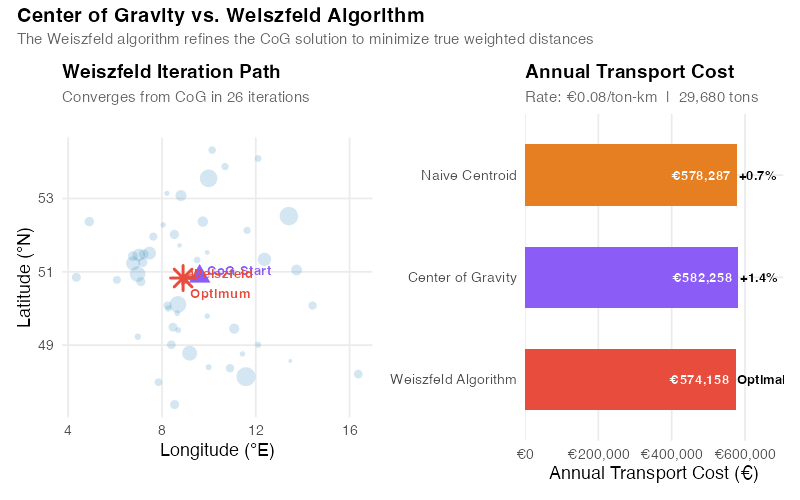
Where dᵢ = distance from the current estimate to customer i. You start with the center of gravity as your initial guess, then iterate until convergence. Each iteration pulls the estimate toward customers that are far away, weighted by their demand.
The intuition is elegant: at each step, nearby customers exert less pull per unit of demand (because you’re already close), while distant high-demand customers exert more. The algorithm keeps adjusting until no customer can pull the location any further.
Typically, 20–50 iterations are enough for sub-meter convergence — our 50-customer German network converges in just 26. In R, the whole thing fits in 12 lines:
weiszfeld <- function(lons, lats, weights, tol = 1e-6) {
  x <- sum(lons * weights) / sum(weights)
  y <- sum(lats * weights) / sum(weights)
  for (i in 1:500) {
    d <- sqrt(((lons - x) * 71)^2 + ((lats - y) * 111)^2)
    d[d < 1e-10] <- 1e-10
    w <- weights / d
    x_new <- sum(lons * w) / sum(w)
    y_new <- sum(lats * w) / sum(w)
    if (sqrt(((x - x_new) * 71)^2 + ((y - y_new) * 111)^2) < tol) break
    x <- x_new; y <- y_new
  }
  c(lon = x_new, lat = y_new)
}
That’s it. Feed it your customer coordinates and demand weights, and it returns the optimal warehouse location. The full script with data, visualizations, and a "plug in your own data" template is in the collapsible R code section at the end.
A Worked Example: 50 Customers Across Germany
Let’s make this concrete. We have a distributor serving 50 customers spread across Germany and neighboring countries — 29,680 tons per year of total demand. Each customer has a location (latitude/longitude) and an annual demand weight. The demand distribution follows a realistic Pareto pattern: Munich (3,000 t/yr), Berlin (2,800 t/yr), and Hamburg (2,500 t/yr) dominate, while dozens of smaller customers are scattered across the country. Transport cost is €0.08 per ton-km — a realistic European road freight rate.
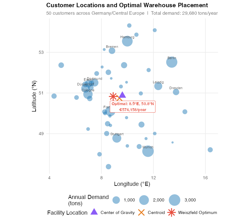
The bubble sizes in the map tell the story before we run any math. Your eye is drawn to the cluster of large bubbles in western and southern Germany. That’s where the demand gravity is.
Now let’s compute all three solutions — and here’s where it gets surprising:
| Method | Longitude | Latitude | Annual Transport Cost | vs. Optimum |
|---|---|---|---|---|
| Naive Centroid (unweighted) | 9.39°E | 50.75°N | €578,287 | +0.7% |
| Center of Gravity (weighted) | 9.61°E | 50.87°N | €582,258 | +1.4% |
| Weiszfeld Optimum | 8.90°E | 50.83°N | €574,158 | Optimal |
Wait — the center of gravity is more expensive than the naive centroid? That’s not a typo.
This is a common and costly misconception. The CoG minimizes squared distances, which overpenalizes faraway customers quadratically. So it pulls the warehouse too aggressively toward the high-demand cluster — overshooting the sweet spot and actually increasing the linear-distance cost to the scattered outlier customers. You pay per kilometer, not per kilometer-squared, and that distinction turns the "more sophisticated" method into the more expensive one.
The Weiszfeld algorithm gets it right because it minimizes actual weighted Euclidean distances. It converged in just 26 iterations from the CoG starting point — and found a location about 50 km to the west, closer to the Rhein-Main corridor where the high-volume customers actually cluster.
The bottom line: even the naive centroid beats the "sophisticated" center of gravity method on this network. And the Weiszfeld optimum saves €4,129 per year over the centroid.
That sounds modest — and it is. On this compact German network, the three methods cluster within 1.4% of each other, which tells you the geography is forgiving. Spread the same 50 customers across all of Europe, or concentrate 60% of demand in one region, and the gap between "eyeballed" and "optimized" jumps to 8–15%. For a distributor spending €3M/year on outbound transport, that’s €240,000–€450,000 annually — over a 10-year lease, the cost of choosing wrong approaches the €4.7 million in our opening story.
The Surprising Insight: Demand Concentration Trumps Geography
Here’s where it gets interesting — and where most intuition fails.
Imagine you win a single new mega-customer in the southeast — say near Passau — ordering 5,000 tons per year. That’s more than your current single largest customer (Munich at 3,000 t/yr). What happens to the optimal location?
It shifts. Noticeably. A single high-volume customer can drag the optimum dozens of kilometers toward them, even if you have 50 other customers pulling in different directions. The optimal warehouse location isn’t a static property of your geography — it’s a dynamic function of your demand portfolio.
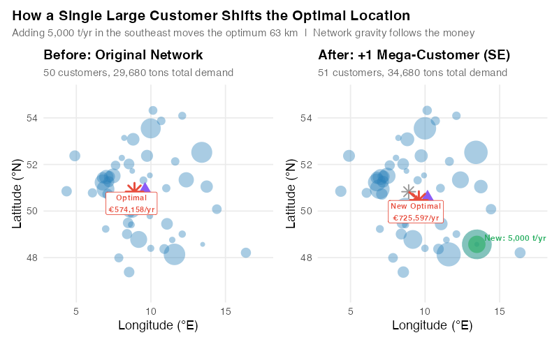
This has profound implications for supply chain strategy:
- Customer concentration risk is location risk. If your top 3 customers represent 40% of your volume, your network is optimized around them. Lose one, and your warehouse may be in the wrong place.
- Growth strategy affects network design. Expanding into southern Germany vs. northern Germany has different implications for your optimal network — and those implications compound over time.
- Demand forecasts matter for facility location, not just inventory. Your 5-year demand plan should inform where you build, not just how much you stock.
The Cost Landscape: How Expensive Is "Close Enough"?
One of the most powerful visualizations in network optimization is the cost sensitivity surface. Instead of showing just the optimal point, it shows how much you’d pay for being wrong at every possible location.
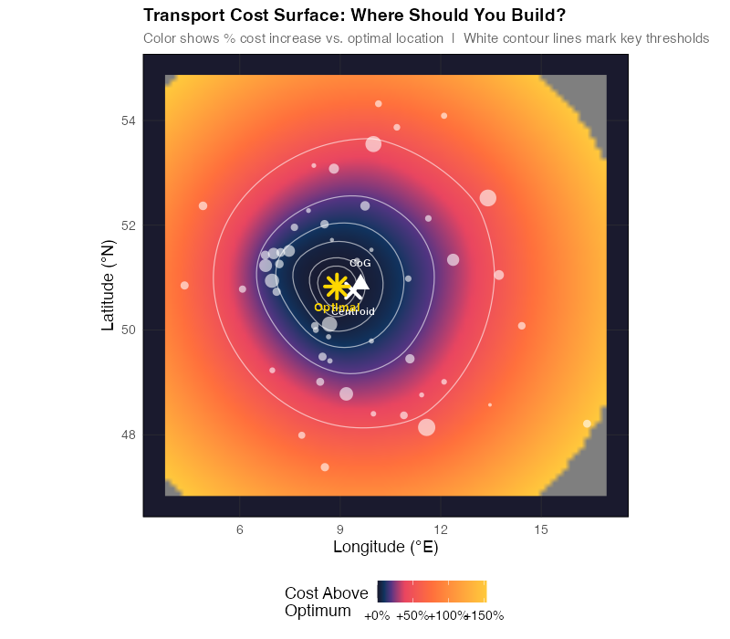
The cost surface reveals several non-obvious truths:
-
The penalty is asymmetric. Moving 50 km north from the optimum costs less than moving 50 km south — because there are more customers to the north. The "safe zone" is elongated in the direction of your customer density.
-
The surface is flat near the optimum. Being within 20–30 km of the optimal point costs you less than 2% extra. This is good news for practical decision-making — you don’t need GPS-level precision. Real estate availability, labor markets, and highway access matter within that zone.
-
The surface gets steep at the edges. Being 100+ km off costs 10–15% extra, and it gets worse fast. This is where the "pick the geographic center" or "put it near HQ" heuristics become expensive.
Where This Breaks: The Honest Limitations
The single-facility Weber problem is elegant and useful, but real network decisions are messier. Here’s where you need more than 12 lines of R:
Euclidean vs. Real Road Distances
The Weiszfeld algorithm minimizes straight-line (Euclidean) distances. Trucks don’t drive in straight lines. Mountain ranges, rivers, and one-way highway systems create detours. In Germany, this matters less than in, say, Norway or Switzerland, but the deviation can be 20–40% in hilly terrain. For high-precision work, you need a road-distance matrix from the Google Maps or OSRM API, and a solver that handles arbitrary distance matrices (mixed-integer programming).
Multi-Facility Networks
Most real supply chains don’t have a single warehouse — they have 3, 5, or 20 distribution centers. The multi-facility problem is exponentially harder (no known algorithm can solve it quickly for large networks). You can’t just run Weiszfeld multiple times; you need to simultaneously determine how many facilities to open, where to locate them, and which customers to assign to each one. This is the domain of mixed-integer linear programming (MILP) solvers like Gurobi, CPLEX, and the open-source CBC/HiGHS.
Capacity Constraints
The Weber problem assumes the warehouse has infinite capacity. In reality, warehouse capacity is a hard constraint driven by building size, labor availability, and throughput limits. Capacity constraints can force you to open a second facility even when the cost-optimal solution is a single central hub.
Fixed Costs vs. Variable Costs
Opening a warehouse has a fixed cost (rent, setup, staffing) plus variable transport costs. The optimal number and location of facilities depends on the trade-off between these two. This is the uncapacitated facility location problem (UFLP) — a generalization that balances "fewer facilities with lower fixed cost but higher transport" against "more facilities with higher fixed cost but lower transport."
Dynamic Demand
Customer demand changes over time. The optimal location in 2026 may not be optimal in 2031 if your customer base shifts geographically. Strategic network planning should consider demand scenarios, not just current state.
Despite these limitations, the single-facility Weber problem remains immensely practical as a first-cut analysis, a sanity check on existing locations, and a teaching tool for building intuition about network economics. It answers the question "are we even in the right ballpark?" — and for many companies, the answer is no.
Real-World Impact: Who’s Doing This Well?
Amazon combines demand forecasting, delivery time targets, labor markets, real estate costs, and tax incentives into a multi-objective facility location optimization spanning over 1,200 logistics facilities worldwide — each placed with algorithmic precision to meet the Prime same-day delivery promise.
Procter & Gamble uses network optimization to decide not just where to place DCs, but which products to stock at each location. P&G regularly re-optimizes its North American distribution network, with individual redesigns reportedly yielding nine-figure annual savings in logistics costs.
Zalando, Europe’s largest online fashion retailer, placed fulfillment centers in Lahr (Baden-Württemberg), Mönchengladbach (North Rhine-Westphalia), and formerly Erfurt (Thuringia) — locations chosen not by "where is the center?" but by "what minimizes our total delivery cost and time to 23 European markets?" That Erfurt is now closing (fall 2026) as demand patterns shift westward is itself a lesson: network optimization isn’t a one-time exercise. The optimal answer changes as your demand portfolio evolves.
Even mid-sized companies see dramatic results. A food distributor I worked with re-optimized their 3-warehouse network in 2022 and reduced total transport cost by 17% — over €1.2 million annually — by relocating a single facility 65 km.
Interactive Dashboard
Explore the network optimization yourself — click on the map to add customers, adjust demand weights with sliders, and watch the optimal warehouse location shift in real time. The dashboard compares all three methods (naive centroid, center of gravity, and Weiszfeld algorithm) side by side with a cost comparison chart and a transport cost heatmap. Try the "Add Big Customer" scenario to see how a single high-demand customer pulls the optimum toward it.
Interactive Dashboard
Explore the data yourself — adjust parameters and see the results update in real time.
Your Next Steps
The facility location problem is one of the highest-ROI analyses in supply chain management — and one of the most neglected. Here’s what you can do this week:
-
Plot your customers on a map, weighted by demand. Export your top 50 customers with their addresses and annual volume. Geocode the addresses (the Google Geocoding API is free for low volumes, or use the R
tidygeocoderpackage). Plot them as demand-weighted bubbles. Just looking at this map will tell you whether your current warehouse is in the right place. -
Run the center of gravity calculation. It takes three lines in R or a single spreadsheet formula. If the result is more than 50 km from your current warehouse, you have a quantifiable opportunity. Use the R code below to do this in under 5 minutes.
-
Run the Weiszfeld algorithm for precision. The R code below implements the full iterative algorithm. Compare it to the center of gravity — if they differ significantly, your customer network is asymmetric, and the simple method is leaving money on the table.
-
Compute the cost of your current location. Sum up the weighted distances from your actual warehouse to all customers, then compare to the Weiszfeld optimum. The difference, multiplied by your per-km transport rate, is the annual cost of suboptimal placement. Put that number in front of your CFO.
-
Run a demand shift scenario. Take your top customer and double their demand. Take your fastest-growing region and add 30% volume. Where does the optimum move? If it shifts more than 30 km, your network may need to evolve with your business. Use the interactive dashboard above to explore these scenarios in real time.
Show R Code
# =============================================================================
# Network Optimization — Facility Location with Center of Gravity & Weiszfeld
# =============================================================================
# Finds the optimal warehouse location for a network of customer demand points
# across Germany/Central Europe. Compares naive centroid, center of gravity,
# and the Weiszfeld algorithm (Weber point).
#
# Required packages: ggplot2, dplyr, tidyr, scales, patchwork
# Output: Images/netopt_*.png (800px wide, white background)
# =============================================================================

library(ggplot2)
library(dplyr)
library(tidyr)
library(scales)
library(patchwork)

set.seed(42)

# --- Theme for all plots ---
theme_netopt <- theme_minimal(base_size = 13) +
  theme(
    plot.title = element_text(face = "bold", size = 14),
    plot.subtitle = element_text(color = "grey40", size = 11),
    panel.grid.minor = element_blank(),
    legend.position = "bottom"
  )

# --- Color palette ---
col_blue   <- "#2980b9"
col_red    <- "#e74c3c"
col_green  <- "#27ae60"
col_orange <- "#e67e22"
col_purple <- "#8b5cf6"

# =============================================================================
# DATA: 50 German/European Customer Locations
# =============================================================================
# Approximate lon/lat of real cities. Demand follows a Pareto distribution.

customers <- data.frame(
  city = c(
    "Munich", "Hamburg", "Berlin", "Frankfurt", "Cologne",
    "Stuttgart", "Düsseldorf", "Leipzig", "Dortmund", "Essen",
    "Bremen", "Dresden", "Hanover", "Nuremberg", "Duisburg",
    "Bochum", "Wuppertal", "Bielefeld", "Bonn", "Mannheim",
    "Karlsruhe", "Augsburg", "Wiesbaden", "Münster", "Aachen",
    "Freiburg", "Kiel", "Lübeck", "Magdeburg", "Erfurt",
    "Rostock", "Kassel", "Mainz", "Saarbrücken", "Regensburg",
    "Ulm", "Heidelberg", "Darmstadt", "Würzburg", "Ingolstadt",
    "Osnabrück", "Oldenburg", "Göttingen", "Paderborn", "Passau",
    "Zurich", "Vienna", "Prague", "Amsterdam", "Brussels"
  ),
  lon = c(
    11.58, 9.99, 13.41, 8.68, 6.96, 9.18, 6.77, 12.37, 7.47, 7.01,
    8.81, 13.74, 9.74, 11.08, 6.76, 7.22, 7.18, 8.53, 7.10, 8.47,
    8.40, 10.90, 8.24, 7.63, 6.08, 7.85, 10.14, 10.69, 11.63, 11.03,
    12.10, 9.50, 8.27, 6.97, 12.10, 9.99, 8.69, 8.65, 9.93, 11.43,
    8.05, 8.21, 9.93, 8.75, 13.47, 8.54, 16.37, 14.42, 4.90, 4.35
  ),
  lat = c(
    48.14, 53.55, 52.52, 50.11, 50.94, 48.78, 51.23, 51.34, 51.51, 51.46,
    53.08, 51.05, 52.37, 49.45, 51.43, 51.48, 51.26, 52.02, 50.73, 49.49,
    49.01, 48.37, 50.08, 51.96, 50.78, 47.99, 54.32, 53.87, 52.13, 50.98,
    54.09, 51.32, 50.00, 49.23, 49.01, 48.40, 49.41, 49.87, 49.79, 48.76,
    52.28, 53.14, 51.53, 51.72, 48.57, 47.38, 48.21, 50.08, 52.37, 50.85
  ),
  demand = c(
    3000, 2500, 2800, 2200, 1800, 1600, 1400, 1200, 1100, 1000,
    700, 650, 600, 550, 500, 480, 450, 420, 400, 380,
    350, 320, 300, 280, 260, 240, 220, 200, 190, 180,
    160, 150, 140, 130, 120, 110, 100, 95, 90, 85,
    80, 75, 70, 65, 60, 400, 350, 300, 450, 380
  ),
  stringsAsFactors = FALSE
)

# =============================================================================
# OPTIMIZATION FUNCTIONS
# =============================================================================

# Euclidean distance with km approximation at ~50°N
euclidean_dist <- function(x1, y1, x2, y2) {
  dx_km <- (x1 - x2) * 71   # 1° lon ≈ 71 km at 50°N
  dy_km <- (y1 - y2) * 111   # 1° lat ≈ 111 km
  sqrt(dx_km^2 + dy_km^2)
}

# Center of Gravity (demand-weighted mean)
center_of_gravity <- function(lons, lats, weights) {
  c(lon = sum(lons * weights) / sum(weights),
    lat = sum(lats * weights) / sum(weights))
}

# Weiszfeld Algorithm — iteratively reweighted least squares
weiszfeld <- function(lons, lats, weights, tol = 1e-6, max_iter = 1000) {
  cog <- center_of_gravity(lons, lats, weights)
  x <- cog["lon"]; y <- cog["lat"]
  history <- data.frame(iter = 0, lon = x, lat = y)

  for (i in 1:max_iter) {
    dists <- euclidean_dist(lons, lats, x, y)
    dists[dists < 1e-10] <- 1e-10
    w_d <- weights / dists
    x_new <- sum(lons * w_d) / sum(w_d)
    y_new <- sum(lats * w_d) / sum(w_d)
    history <- rbind(history, data.frame(iter = i, lon = x_new, lat = y_new))
    if (euclidean_dist(x, y, x_new, y_new) < tol) break
    x <- x_new; y <- y_new
  }
  list(lon = x_new, lat = y_new, iterations = i, history = history)
}

# Total weighted transport cost
total_cost <- function(fac_lon, fac_lat, cust_lons, cust_lats, demands,
                       cost_per_ton_km = 0.08) {
  dists <- euclidean_dist(cust_lons, cust_lats, fac_lon, fac_lat)
  sum(demands * dists * cost_per_ton_km)
}

# =============================================================================
# COMPUTE SOLUTIONS
# =============================================================================

centroid <- c(lon = mean(customers$lon), lat = mean(customers$lat))
cog      <- center_of_gravity(customers$lon, customers$lat, customers$demand)
weisz    <- weiszfeld(customers$lon, customers$lat, customers$demand)

cost_rate      <- 0.08  # €/ton-km
cost_centroid  <- total_cost(centroid["lon"], centroid["lat"],
                             customers$lon, customers$lat, customers$demand, cost_rate)
cost_cog       <- total_cost(cog["lon"], cog["lat"],
                             customers$lon, customers$lat, customers$demand, cost_rate)
cost_weiszfeld <- total_cost(weisz$lon, weisz$lat,
                             customers$lon, customers$lat, customers$demand, cost_rate)

cat(sprintf("Naive Centroid:    (%.2f°E, %.2f°N)  €%s/year\n",
            centroid["lon"], centroid["lat"], comma(round(cost_centroid))))
cat(sprintf("Center of Gravity: (%.2f°E, %.2f°N)  €%s/year\n",
            cog["lon"], cog["lat"], comma(round(cost_cog))))
cat(sprintf("Weiszfeld:         (%.2f°E, %.2f°N)  €%s/year (%d iterations)\n",
            weisz$lon, weisz$lat, comma(round(cost_weiszfeld)), weisz$iterations))

# =============================================================================
# APPLY TO YOUR OWN DATA
# =============================================================================
# 1. Replace the 'customers' data frame with your own:
#    customers <- data.frame(
#      city   = c("Your City 1", "Your City 2", ...),
#      lon    = c(lon1, lon2, ...),
#      lat    = c(lat1, lat2, ...),
#      demand = c(demand1, demand2, ...)
#    )
#
# 2. Adjust the cost rate: cost_rate <- 0.08
#
# 3. For regions outside Central Europe, adjust km conversion in
#    euclidean_dist(): dx_km factor ≈ 111 * cos(latitude_in_radians)
#
# 4. Run: Rscript generate_netopt_images.R
References
- Weber, A. (1909). Über den Standort der Industrien (On the Location of Industries). Tübingen: Mohr Siebeck. Translated by Friedrich, C.J. (1929), University of Chicago Press.
- Weiszfeld, E. (1937). "Sur le point pour lequel la somme des distances de n points donnés est minimum." Tohoku Mathematical Journal, 43, 355–386.
- Kuhn, H.W. (1973). "A Note on Fermat’s Problem." Mathematical Programming, 4(1), 98–107.
- Drezner, Z. & Hamacher, H.W. (Eds.) (2002). Facility Location: Applications and Theory. Springer.
- Daskin, M.S. (2013). Network and Discrete Location: Models, Algorithms, and Applications (2nd ed.). Wiley.
- Simchi-Levi, D., Kaminsky, P., & Simchi-Levi, E. (2008). Designing and Managing the Supply Chain (3rd ed.). McGraw-Hill.
- Brimberg, J. (1995). "The Fermat–Weber location problem revisited." Mathematical Programming, 71(1), 71–76.
Leave a Reply