€340,000 Hiding in Plain Sight
Typical slow-mover inventory data. 1,200 SKUs with annual demand under 100 units. Average MOQ from suppliers: 500 pieces.
That means for those 1,200 items, you order 5x what you need — then store the excess for years. Some of it expires. Some becomes obsolete. Most of it just sits there, quietly eating working capital at 25 cents on the euro per year.
The total cost of excess inventory from MOQ overbuys? Roughly €340,000 per year. Nobody had ever calculated it. It wasn’t in any report. It didn’t trigger any alert in the ERP. The system just did what it was told: order the minimum. The minimum was too much.
This number shouldn’t surprise anyone who manages procurement. MOQs are set once, stored in the item master, and left untouched for years while the world around them changes — demand drops, products phase out, better suppliers emerge. But nobody reviews them because they look like a constraint, not a decision. They sit in that “supplier says so” category of things we stop questioning.
That’s a mistake. And in this post, I’ll show you exactly how much it’s costing you — with a dataset of 30 SKUs, the math to quantify the damage, and three strategies that actually work to fix it.
What MOQs Really Are (And What They’re Not)
Here’s the thing most buyers miss about MOQs: suppliers don’t set them because that’s the smallest quantity they can produce. They set them because that’s the smallest quantity they want to produce. Those are two very different things.
MOQs protect the supplier’s setup costs, their batch economics, their production scheduling convenience. A supplier running injection-molded plastic parts might need 20 minutes to change a tool. At €150/hour for machine time, that’s €50 in changeover cost. If the part sells for €2, the supplier needs to spread that €50 across enough units to maintain their margin — so they set an MOQ of 500 pieces and move on.
But here’s what the supplier won’t volunteer: that €50 changeover cost is fixed. Whether the MOQ is 500 or 250 or 100, the setup cost is still €50. The MOQ isn’t the break-even point for the supplier — it’s the comfort point. It’s the quantity where the per-unit overhead contribution is so small that the supplier’s sales team doesn’t have to think about it.
MOQs are a negotiation position, not a law of physics.
Once you understand this, three things become clear:
- MOQs are negotiable — because they’re set for convenience, not survival
- The supplier knows the setup cost — they just haven’t shared it with you
- You’re paying for their convenience — in carrying cost, obsolescence risk, and tied-up working capital
The Hidden Cost Formula
The cost of an MOQ overbuy is straightforward to calculate, yet almost nobody does it. Here’s the formula:
Annual Excess Carrying Cost = (MOQ − Annual Demand) × Unit Cost × Holding Rate
Where:
- MOQ is the minimum order quantity set by the supplier
- Annual Demand is what you actually use per year
- Unit Cost is the purchase price per unit
- Holding Rate is the annual cost of holding inventory as a percentage of its value (typically 20–30% for industrial goods, covering warehousing, insurance, capital cost, shrinkage, and obsolescence)
Note: this formula assumes demand is low enough that the MOQ covers more than one year of demand. When MOQ > annual demand, you’re sitting on excess for the full year — or longer. When MOQ < annual demand but isn’t a clean multiple, the excess is smaller but still real. We’ll focus on the first case because that’s where the pain is concentrated.
Worked Example: A Single SKU
Take a hydraulic fitting — a standard catalog part that goes into industrial equipment:
| Parameter | Value |
|---|---|
| Supplier MOQ | 500 units |
| Annual demand | 80 units |
| Unit cost | €12.50 |
| Holding rate | 25% per year |
Excess units per order: 500 − 80 = 420 units
Cost of excess: 420 × €12.50 × 0.25 = €1,312.50 per year
For a €12.50 part. On a single SKU. The purchase price for the entire MOQ is €6,250 — and you’re paying an invisible 21% surcharge just to hold the stuff you don’t need.
Now multiply that across hundreds of slow-moving SKUs. The numbers get alarming fast.
30 SKUs That Tell the Story
To make this concrete, I built a dataset of 30 representative parts — the kind of items you’d find in any industrial procurement portfolio. These aren’t exotic components; they’re the brackets, gaskets, connectors, and fasteners that fill warehouses everywhere.
The dataset captures real-world patterns: MOQs that range from 200 to 2,000, demands from 15 to 450, and unit costs from €1.50 to €85. Every number is realistic; the patterns are drawn from actual procurement data across multiple industries.
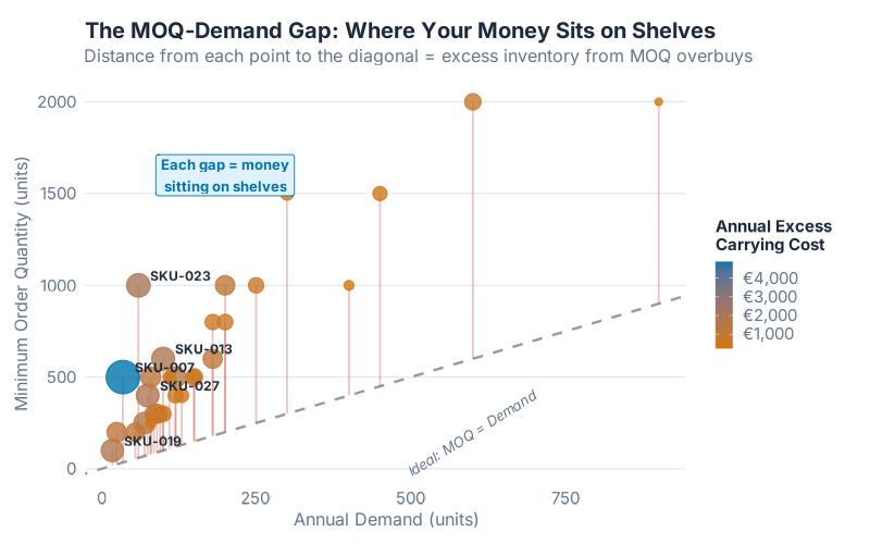
The scatter plot tells the story at a glance. Each dot is a SKU. The diagonal line represents the ideal state: MOQ equals demand, zero waste. Every dot above that line is money sitting on shelves. The further above the line, the bigger the problem.
Some highlights from the data:
| SKU | Description | MOQ | Annual Demand | Excess Units | Unit Cost | Annual Carrying Cost |
|---|---|---|---|---|---|---|
| SKU-007 | Stainless steel bearing | 500 | 35 | 465 | €42.00 | €4,882.50 |
| SKU-023 | Titanium fastener set | 1,000 | 60 | 940 | €8.50 | €1,997.50 |
| SKU-013 | Cast iron flange | 600 | 100 | 500 | €15.00 | €1,875.00 |
| SKU-027 | Phosphor bronze spring | 400 | 75 | 325 | €22.50 | €1,828.13 |
| SKU-019 | Precision servo motor | 100 | 18 | 82 | €85.00 | €1,742.50 |
The top five offenders alone account for over €12,000 per year in carrying costs. And these are just 30 SKUs out of thousands.
The Pareto of Pain: Finding Your MOQ Offenders
Not all MOQ overbuys are created equal. A €1.50 rubber gasket with an MOQ of 1,000 and demand of 200 costs you €300/year in excess carrying cost — annoying but manageable. A €42.00 stainless steel bearing with an MOQ of 500 and demand of 35 costs you almost €5,000/year — that’s a problem worth solving.
The Pareto chart below ranks all 30 SKUs by their annual excess carrying cost. The pattern is familiar to anyone in procurement: a small number of items drive the majority of the waste.
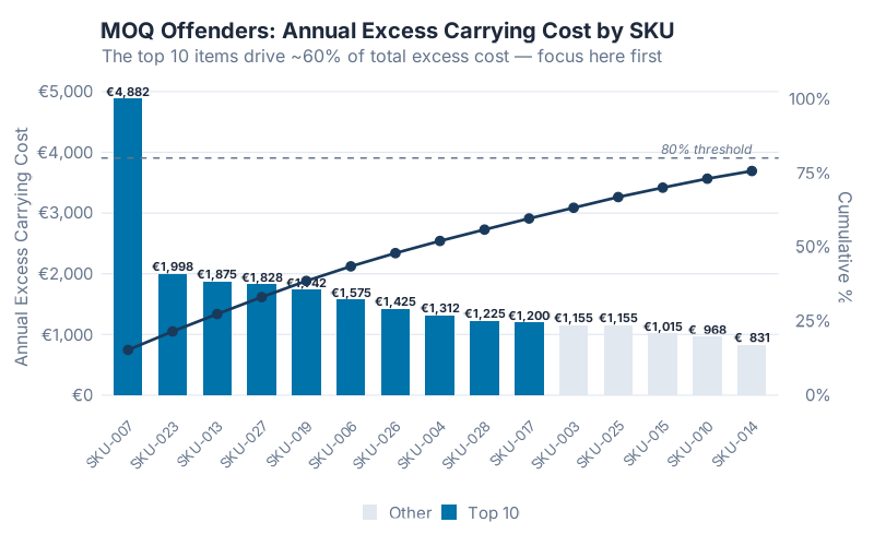
The top 10 MOQ offenders drive approximately 60% of total excess carrying cost across all 30 SKUs. This is your hit list. These are the items where renegotiating the MOQ — or finding alternative strategies — will have the biggest impact on working capital.
How to identify your MOQ offenders in practice:
- Export your item master data: SKU, MOQ, annual demand (or trailing 12-month usage), and unit cost
- Calculate excess carrying cost for each item: (MOQ − demand) × unit cost × holding rate
- Sort descending by carrying cost
- Focus on the top 50 — that’s one afternoon of analysis for potentially six figures of savings
Most ERP systems can produce this report in minutes. The obstacle isn’t technical; it’s that nobody asks the question.
Three Strategies That Actually Work
Strategy 1: Calculate Before You Capitulate
Before accepting any MOQ, calculate what it really costs you. This sounds obvious, but in practice, buyers negotiate the unit price and accept the MOQ as a given. Flipping that order — evaluate the MOQ cost first, then decide whether the unit price justifies it — changes everything.
The decision rule: If the annual excess carrying cost exceeds what you’d save by ordering from this supplier versus the next-best alternative, the MOQ is too high. Walk, negotiate, or find another path.
For the hydraulic fitting example:
- Supplier A: €12.50/unit, MOQ 500 → excess carrying cost = €1,312.50/year
- Supplier B: €14.00/unit, MOQ 100 → excess carrying cost = €70.00/year
- Annual spend at Supplier A: 80 × €12.50 = €1,000
- Annual spend at Supplier B: 80 × €14.00 = €1,120
- Net cost difference: €120 more on unit price, but €1,242.50 less in carrying cost
Supplier B is €1,122.50/year cheaper despite a higher unit price. But you’d never see that by comparing quotes on price alone.
Strategy 2: Consolidate, Don’t Capitulate (Joint Replenishment)
If a supplier’s MOQ is 500 and you need 80 — check whether three other items from the same supplier have the same problem. Bundle them. Hit the supplier’s economic threshold without overstocking any single part.
This is the Joint Replenishment Problem (JRP) in operations research, and it’s one of the most underused levers in procurement.
The idea is simple: suppliers set MOQs partly to cover their fixed costs per order (order processing, changeover, shipping setup). If you can combine multiple SKUs into a single purchase order that collectively meets the supplier’s minimum order value rather than a per-SKU minimum quantity, everyone wins:
- The supplier gets the order size they need for economic production
- You avoid overstocking on any individual SKU
- Order processing costs drop because you’re placing one PO instead of four
Example: You buy four items from Supplier C, each with an MOQ of 500 units:
| Item | MOQ | Your Demand | If Ordered Separately |
|---|---|---|---|
| Part A | 500 | 120 | 380 excess units |
| Part B | 500 | 200 | 300 excess units |
| Part C | 500 | 80 | 420 excess units |
| Part D | 500 | 150 | 350 excess units |
Separately: 1,450 excess units across four SKUs.
Consolidated: One combined order of 550 units total (120 + 200 + 80 + 150), worth more to the supplier than four micro-orders. Negotiate a combined minimum order value instead of per-SKU MOQs. Excess units: zero.
Note: this works best with distributors and suppliers whose MOQs are driven by order processing costs rather than per-part tooling. For manufacturers with production-driven MOQs (tooling changes, extrusion setups), per-SKU minimums may have a genuine physical basis. In those cases, Strategy 3 is usually more effective.
Strategy 3: Ask for the Setup Cost, Then Offer a Surcharge
This is the strategy that most procurement professionals have never tried — and it’s often the most effective.
When you know the supplier’s actual changeover cost, you can offer to pay a small premium per unit on short runs instead of accepting a 500-piece minimum. The math almost always favors the surcharge.
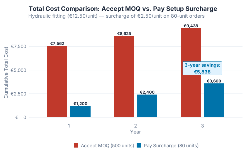
Worked example:
| Scenario | Accept MOQ (500 units) | Pay Surcharge (80 units) |
|---|---|---|
| Units ordered | 500 | 80 |
| Unit cost | €12.50 | €12.50 + €2.50 surcharge = €15.00 |
| Purchase cost | €6,250 | €1,200 |
| Setup cost absorbed | Included in unit price | €200 (passed through as surcharge) |
| Excess units | 420 | 0 |
| Year 1 carrying cost | €1,312.50 (420 excess units) | €0 |
| Year 2 carrying cost | €1,062.50 (340 excess units) | €0 |
| Year 3 carrying cost | €812.50 (260 excess units) | €0 |
| Year 1 total cost | €7,562.50 | €1,200 |
| 3-year total cost | €9,437.50 | €3,600 |
Over three years, the surcharge approach saves €5,837.50 — on a single SKU. The unit price is 20% higher, but the total cost is 62% lower.
The key insight: a €2.50/unit surcharge on 80 units costs you €200 — exactly the supplier’s changeover cost. You’re paying it either way; the question is whether you also pay €1,312.50/year to warehouse 420 units you don’t need.
How to execute this conversation:
- Ask the supplier: “What’s your actual changeover or setup cost for this part?”
- Most suppliers will answer — it’s not confidential, it’s operational
- Divide the setup cost by your order quantity to get the per-unit surcharge
- Present the comparison: “We can pay €15/unit for 80 pieces, or you can keep the MOQ at 500 and we’ll source from Supplier B”
When MOQs Make Sense (And When They Don’t)
Not every MOQ is a problem. MOQs are reasonable when:
- Demand is close to the MOQ — if you need 450 and the MOQ is 500, the excess is trivial
- The item is cheap and stable — a €0.50 O-ring with a 1,000-piece MOQ costs €125/year in excess carrying. Not worth fighting over.
- The item has a long shelf life and stable demand — you’ll use it eventually, and the carrying cost is just a timing cost, not a waste cost
- There’s a genuine physical minimum — chemical batches, extrusion runs, or printed circuit board panels sometimes do have real production minimums
One trade-off to keep in mind: ordering smaller quantities more frequently means more reorder cycles and more exposure to lead time variability. Factor in any additional safety stock requirements when comparing total cost — the carrying cost savings from lower MOQs should outweigh any increase in safety stock.
MOQs are a problem when:
- The MOQ-to-demand ratio is 3:1 or higher — you’re ordering triple what you need
- The item is expensive — high unit cost amplifies carrying cost
- Demand is declining or uncertain — that excess may never be used
- The item has obsolescence risk — engineering changes, product phase-outs, or shelf life limits turn excess inventory into scrap
The Sensitivity Landscape: Where MOQ Costs Bite Hardest
The carrying cost of an MOQ overbuy depends on two factors that multiply together: unit cost and the size of the excess. The heatmap below shows how annual carrying cost changes across different unit prices and demand levels (holding MOQ constant at 500 and holding rate at 25%).
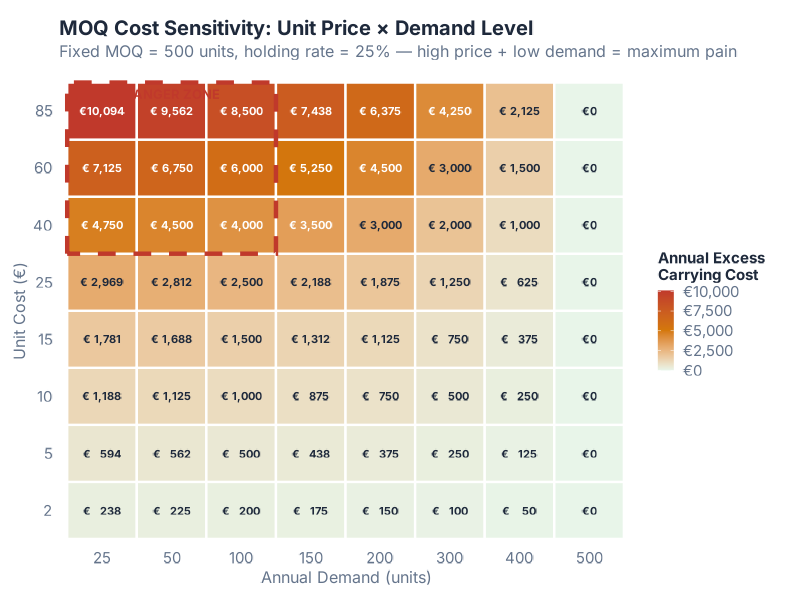
The pattern is clear: high unit cost + low demand = maximum pain. The upper-left corner of the heatmap is where your worst MOQ offenders live. These are the SKUs where renegotiation has the highest payoff — and they’re often overlooked because buyers focus on high-volume, high-spend items in their ABC analysis.
This is the blind spot in traditional procurement analytics. ABC analysis ranks items by total spend — but total spend is a function of price × volume. A €85 precision motor with demand of 18 units barely registers on an ABC spend report (€1,530/year). But its MOQ excess costs €1,742.50/year in carrying — more than the annual purchase spend. Traditional ABC analysis will never flag this item. MOQ analysis will.
Building a Quarterly MOQ Review Process
Finding your MOQ offenders once is useful. Making it a habit is transformative. Here’s a practical process that takes one afternoon per quarter and typically finds five to six figures of savings.
Step 1: Extract the data (15 minutes)
Pull from your ERP: SKU, description, supplier, MOQ, trailing 12-month demand, unit cost, and last order date. Most systems can produce this in a standard report or a simple query.
Step 2: Calculate the excess (15 minutes)
For each SKU: excess carrying cost = max(0, MOQ − annual demand) × unit cost × holding rate. Use 25% as the holding rate if you don’t have a company-specific number — it’s the industry standard for industrial goods.
Step 3: Rank and filter (15 minutes)
Sort by excess carrying cost descending. Filter to the top 50. These are your MOQ offenders for this quarter.
Step 4: Classify and act (2 hours)
For each of the top 50, assign one of four actions:
| Action | When to Use | Expected Outcome |
|---|---|---|
| Renegotiate MOQ | Supplier relationship is strong; you have leverage | Lower MOQ, same or similar unit price |
| Offer surcharge | Supplier’s setup cost is known or discoverable | Pay per-unit premium, eliminate excess |
| Consolidate orders | Multiple low-volume SKUs from same supplier | Combined order meets supplier threshold |
| Switch supplier | Alternative exists with lower or no MOQ | Eliminate the problem entirely |
Step 5: Track results (ongoing)
Measure the before-and-after: total excess carrying cost this quarter versus last quarter. The chart below shows the typical impact of a structured MOQ optimization program.
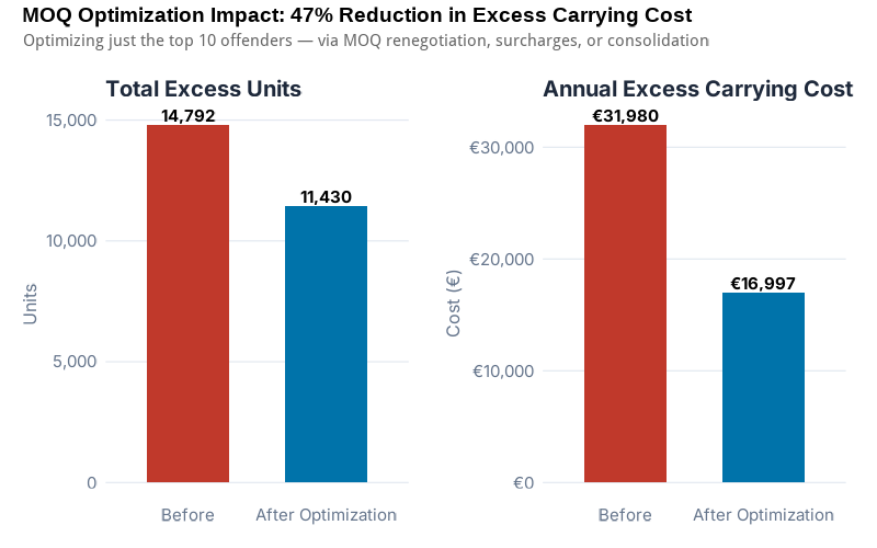
In our 30-SKU portfolio, applying these strategies to just the top 10 offenders reduces total excess carrying cost by approximately 47% — without changing a single unit price. The savings come entirely from ordering what you need instead of what the supplier’s MOQ dictates.
Key Takeaways
- MOQs are a negotiation position, not a constraint. Suppliers set them for their convenience — to cover setup costs and simplify production scheduling. Understanding this shifts the conversation from “Can we get a lower MOQ?” to “What’s your setup cost, and how can we share it fairly?”
- The hidden cost formula is simple but devastating. (MOQ − Demand) × Unit Cost × Holding Rate. Run this calculation on your slow-movers and you’ll find five to six figures of invisible cost. The data is already in your ERP — nobody’s asking the question.
- Unit price comparison is incomplete without MOQ analysis. A supplier with a lower price but a higher MOQ can easily be more expensive in total cost. Always compare total cost of ownership, including the carrying cost of excess inventory.
- Three strategies cover most situations. Calculate the true cost before accepting (Strategy 1). Consolidate orders across SKUs from the same supplier (Strategy 2). Ask for the setup cost and offer a per-unit surcharge (Strategy 3). Most procurement teams use none of these; the best teams use all three.
- Focus on the top 50 offenders. Pareto applies: a small number of SKUs drive the majority of excess carrying cost. One afternoon per quarter reviewing these items will find more savings than a month of unit-price negotiations.
Your Next Steps
- Run the MOQ offender report this week. Export your item master, calculate excess carrying cost, and sort descending. The R code below automates this, but a pivot table works fine too. Focus on items where MOQ exceeds annual demand by 3x or more.
- Pick your top 5 offenders and calculate the surcharge alternative. For each one, estimate the supplier’s setup cost (or ask them directly). Compare: total cost of accepting the MOQ versus total cost of paying a per-unit surcharge on a short run. The numbers will make the business case for you.
- Schedule a quarterly MOQ review. Block two hours every quarter to refresh the analysis. Demand changes, suppliers change, and MOQs that made sense two years ago may be costing you thousands today.
- Use the interactive dashboard below to plug in your own SKUs and compare strategies in real time. It calculates excess carrying cost, surcharge break-even points, and projected savings — so you walk into your next supplier meeting with numbers, not feelings.
Interactive Dashboard
Explore the data yourself — input your unit costs, MOQs, actual demand, and holding rate to compare strategies and find your biggest MOQ offenders.
Interactive Dashboard
Explore the data yourself — adjust parameters and see the results update in real time.
Show R Code
# =============================================================================
# MOQ Hidden Cost Analysis
# =============================================================================
# Analyzes the hidden carrying costs of Minimum Order Quantity (MOQ) overbuys,
# identifies the worst offenders, and compares mitigation strategies.
#
# To adapt to your own data:
# 1. Replace the sample dataset in the DATA SETUP section with your own SKUs
# 2. Adjust the holding_rate if your company uses a different value
# 3. Run the full script — all charts and analysis update automatically
#
# Required packages: ggplot2, dplyr, tidyr, scales, patchwork
# =============================================================================

library(ggplot2)
library(dplyr)
library(tidyr)
library(scales)
library(patchwork)

# --- Theme for all plots ---
theme_moq <- theme_minimal(base_size = 13) +
  theme(
    plot.title = element_text(face = "bold", size = 14),
    plot.subtitle = element_text(color = "grey40", size = 11),
    panel.grid.minor = element_blank(),
    legend.position = "bottom"
  )

# Color palette
moq_colors <- c(
  excess = "#e74c3c",
  demand = "#27ae60",
  neutral = "#2980b9",
  highlight = "#f39c12",
  dark = "#2c3e50",
  light = "#ecf0f1"
)

# =============================================================================
# 1. DATA SETUP — 30 representative SKUs
# =============================================================================

holding_rate <- 0.25  # 25% annual holding cost

skus <- data.frame(
  sku = paste0("SKU-", sprintf("%03d", 1:30)),
  description = c(
    "Carbon steel bracket",       "Nylon cable gland",
    "Aluminum heat sink",         "Hydraulic fitting",
    "Silicone gasket set",        "Copper bus bar",
    "Stainless steel bearing",    "Rubber vibration mount",
    "Brass compression fitting",  "Polyurethane roller",
    "Spring steel clip",          "PTFE seal ring",
    "Cast iron flange",           "Zinc alloy housing",
    "Ceramic insulator",          "Neoprene O-ring kit",
    "Hardened steel pin",         "Fiberglass spacer",
    "Precision servo motor",      "Anodized end cap",
    "Stainless hose clamp",       "Acetal gear wheel",
    "Titanium fastener set",      "Nickel plated contact",
    "Delrin bushing",             "Viton seal kit",
    "Phosphor bronze spring",     "Control valve assembly",
    "LED indicator module",       "Epoxy potting compound"
  ),
  supplier = rep(c("Supplier A", "Supplier B", "Supplier C",
                    "Supplier D", "Supplier E"), each = 6),
  moq = c(
    500, 1000, 300, 500, 2000, 250,
    500, 1000, 400, 300, 1500, 800,
    600, 500, 200, 2000, 1000, 500,
    100, 400, 1500, 300, 1000, 800,
    600, 500, 400, 200, 300, 250
  ),
  annual_demand = c(
    150, 400, 90,  80,  600, 70,
    35,  250, 120, 85,  300, 180,
    100, 150, 55,  900, 200, 110,
    18,  130, 450, 95,  60,  200,
    180, 120, 75,  25,  100, 80
  ),
  unit_cost = c(
    5.50,  1.80,  22.00, 12.50, 2.20,  35.00,
    42.00, 3.50,  8.75,  18.00, 1.50,  4.20,
    15.00, 9.50,  28.00, 0.85,  6.00,  3.80,
    85.00, 7.50,  2.00,  12.00, 8.50,  4.50,
    11.00, 15.00, 22.50, 28.00, 14.00, 6.50
  ),
  stringsAsFactors = FALSE
)

# =============================================================================
# 2. CALCULATE EXCESS COSTS
# =============================================================================

skus <- skus %>%
  mutate(
    excess_units = pmax(0, moq - annual_demand),
    excess_cost  = excess_units * unit_cost * holding_rate,
    moq_demand_ratio = moq / annual_demand,
    excess_pct = excess_units / moq * 100
  ) %>%
  arrange(desc(excess_cost))

# Print summary
cat("=== MOQ HIDDEN COST ANALYSIS ===\n\n")
cat(sprintf("Total SKUs analyzed: %d\n", nrow(skus)))
cat(sprintf("Total annual excess carrying cost: €%s\n",
            format(sum(skus$excess_cost), big.mark = ",", digits = 0, nsmall = 2)))
cat(sprintf("Average MOQ-to-demand ratio: %.1fx\n", mean(skus$moq_demand_ratio)))
cat(sprintf("SKUs where MOQ > 3x demand: %d\n\n",
            sum(skus$moq_demand_ratio > 3)))

top10_pct <- round(sum(head(skus, 10)$excess_cost) / sum(skus$excess_cost) * 100)
cat(sprintf("Top 10 share of total: %d%%\n\n", top10_pct))

cat("Top 10 MOQ Offenders:\n")
print(skus %>%
        head(10) %>%
        select(sku, description, moq, annual_demand, excess_units,
               unit_cost, excess_cost) %>%
        mutate(excess_cost = sprintf("€%.2f", excess_cost)))

# =============================================================================
# 3. CHART 1 — MOQ vs. Demand Scatter (Excess Inventory Gap)
# =============================================================================

p1 <- ggplot(skus, aes(x = annual_demand, y = moq)) +
  # Diagonal reference line: MOQ = Demand (ideal)
  geom_abline(slope = 1, intercept = 0, linetype = "dashed",
              color = "grey60", linewidth = 0.8) +
  # Segments from each point down to the diagonal
  geom_segment(aes(xend = annual_demand, yend = annual_demand),
               color = moq_colors["excess"], alpha = 0.3, linewidth = 0.6) +
  # Points colored by excess cost
  geom_point(aes(size = excess_cost, color = excess_cost), alpha = 0.8) +
  scale_color_gradient(low = moq_colors["highlight"], high = moq_colors["excess"],
                       labels = label_dollar(prefix = "€"),
                       name = "Annual Excess\nCarrying Cost") +
  scale_size_continuous(range = c(2, 10), guide = "none") +
  # Label the worst offenders
  geom_text(data = skus %>% head(5),
            aes(label = sku), hjust = -0.2, vjust = -0.5,
            size = 3.2, fontface = "bold", color = moq_colors["dark"]) +
  # Annotation
  annotate("text", x = 600, y = 200, label = "Ideal: MOQ = Demand",
           color = "grey50", size = 3.5, fontface = "italic", angle = 32) +
  annotate("label", x = 50, y = 1800,
           label = "Each gap = money\nsitting on shelves",
           fill = "#fff3e0", color = moq_colors["excess"],
           size = 3.5, fontface = "bold", label.size = 0.5) +
  labs(
    title = "The MOQ-Demand Gap: Where Your Money Sits on Shelves",
    subtitle = "Distance from each point to the diagonal = excess inventory from MOQ overbuys",
    x = "Annual Demand (units)",
    y = "Minimum Order Quantity (units)"
  ) +
  theme_moq +
  theme(legend.position = "right")

ggsave("https://inphronesys.com/wp-content/uploads/2026/03/moq_excess_inventory_gap-2.png", p1,
       width = 8, height = 5, dpi = 100, bg = "white")

# =============================================================================
# 4. CHART 2 — Top Offenders Pareto Chart
# =============================================================================

skus_ranked <- skus %>%
  mutate(
    rank = row_number(),
    cumulative_cost = cumsum(excess_cost),
    cumulative_pct = cumulative_cost / sum(excess_cost) * 100
  )

# Show top 15 for readability
top_n <- 15
skus_top <- skus_ranked %>% head(top_n)

p2 <- ggplot(skus_top, aes(x = reorder(sku, -excess_cost), y = excess_cost)) +
  geom_col(aes(fill = ifelse(rank <= 10, "Top 10", "Other")),
           width = 0.7) +
  geom_text(aes(label = sprintf("€%s", format(round(excess_cost), big.mark = ","))),
            vjust = -0.3, size = 3, fontface = "bold") +
  # Cumulative line on secondary axis
  geom_line(aes(y = cumulative_pct / 100 * max(skus_top$excess_cost),
                group = 1),
            color = moq_colors["dark"], linewidth = 1, linetype = "solid") +
  geom_point(aes(y = cumulative_pct / 100 * max(skus_top$excess_cost)),
             color = moq_colors["dark"], size = 2) +
  # 80% threshold line
  geom_hline(yintercept = 80 / 100 * max(skus_top$excess_cost),
             linetype = "dotted", color = "grey50") +
  annotate("text", x = top_n - 1, y = 82 / 100 * max(skus_top$excess_cost),
           label = "80% of total cost", color = "grey50", size = 3,
           fontface = "italic") +
  scale_fill_manual(values = c("Top 10" = moq_colors["excess"],
                                "Other" = moq_colors["highlight"]),
                    name = NULL) +
  scale_y_continuous(
    labels = label_dollar(prefix = "€"),
    sec.axis = sec_axis(~ . / max(skus_top$excess_cost) * 100,
                        name = "Cumulative %",
                        labels = label_percent(scale = 1))
  ) +
  labs(
    title = "MOQ Offenders: Annual Excess Carrying Cost by SKU",
    subtitle = sprintf("The top 10 items drive ~%d%% of total excess cost — focus here first",
                        top10_pct),
    x = NULL,
    y = "Annual Excess Carrying Cost"
  ) +
  theme_moq +
  theme(axis.text.x = element_text(angle = 45, hjust = 1, size = 10))

ggsave("https://inphronesys.com/wp-content/uploads/2026/03/moq_top_offenders-2.png", p2,
       width = 8, height = 5, dpi = 100, bg = "white")

# =============================================================================
# 5. CHART 3 — Strategy Comparison: MOQ vs. Surcharge
# =============================================================================

# Compare 3-year total cost for a representative SKU (hydraulic fitting)
years <- 1:3
moq_qty <- 500
demand <- 80
unit_cost_base <- 12.50
surcharge <- 2.50
setup_cost <- 200

strategy_data <- data.frame(
  year = rep(years, 2),
  strategy = rep(c("Accept MOQ (500 units)", "Pay Surcharge (80 units)"), each = 3),
  purchase_cost = c(
    # MOQ: buy 500 in year 1, nothing in years 2-3 (excess covers demand)
    moq_qty * unit_cost_base, 0, 0,
    # Surcharge: buy 80 each year
    rep(demand * (unit_cost_base + surcharge), 3)
  ),
  carrying_cost = c(
    # MOQ: carrying cost on declining excess
    (moq_qty - demand * 1) * unit_cost_base * holding_rate,
    (moq_qty - demand * 2) * unit_cost_base * holding_rate,
    (moq_qty - demand * 3) * unit_cost_base * holding_rate,
    # Surcharge: no excess
    0, 0, 0
  )
) %>%
  mutate(
    total_cost = purchase_cost + carrying_cost,
    cumulative = ave(total_cost, strategy, FUN = cumsum)
  )

p3 <- ggplot(strategy_data, aes(x = factor(year), y = cumulative,
                                 fill = strategy)) +
  geom_col(position = position_dodge(width = 0.7), width = 0.6) +
  geom_text(aes(label = sprintf("€%s", format(round(cumulative), big.mark = ","))),
            position = position_dodge(width = 0.7),
            vjust = -0.3, size = 3.5, fontface = "bold") +
  scale_fill_manual(values = c("Accept MOQ (500 units)" = moq_colors["excess"],
                                "Pay Surcharge (80 units)" = moq_colors["demand"]),
                    name = NULL) +
  scale_y_continuous(labels = label_dollar(prefix = "€")) +
  # Savings annotation
  annotate("label", x = 3, y = max(strategy_data$cumulative) * 0.55,
           label = sprintf("3-year savings:\n€%s",
                           format(round(
                             sum(strategy_data$cumulative[strategy_data$strategy ==
                               "Accept MOQ (500 units)" & strategy_data$year == 3]) -
                             sum(strategy_data$cumulative[strategy_data$strategy ==
                               "Pay Surcharge (80 units)" & strategy_data$year == 3])
                           ), big.mark = ",")),
           fill = "#e8f5e9", color = moq_colors["demand"],
           size = 4, fontface = "bold", label.size = 0.5) +
  labs(
    title = "Total Cost Comparison: Accept MOQ vs. Pay Setup Surcharge",
    subtitle = "Hydraulic fitting (€12.50/unit) — surcharge of €2.50/unit on 80-unit orders",
    x = "Year",
    y = "Cumulative Total Cost"
  ) +
  theme_moq

ggsave("https://inphronesys.com/wp-content/uploads/2026/03/moq_cost_comparison-2.png", p3,
       width = 8, height = 5, dpi = 100, bg = "white")

# =============================================================================
# 6. CHART 4 — Sensitivity Heatmap: Unit Price × Demand Level
# =============================================================================

# Fixed MOQ = 500, holding rate = 25%
moq_fixed <- 500
unit_prices <- c(2, 5, 10, 15, 25, 40, 60, 85)
demand_levels <- c(25, 50, 100, 150, 200, 300, 400, 500)

sensitivity <- expand.grid(
  unit_price = unit_prices,
  demand = demand_levels
) %>%
  mutate(
    excess = pmax(0, moq_fixed - demand),
    carrying_cost = excess * unit_price * holding_rate,
    label = ifelse(carrying_cost > 0,
                   sprintf("€%s", format(round(carrying_cost), big.mark = ",")),
                   "€0")
  )

p4 <- ggplot(sensitivity, aes(x = factor(demand), y = factor(unit_price),
                               fill = carrying_cost)) +
  geom_tile(color = "white", linewidth = 0.8) +
  geom_text(aes(label = label),
            size = 3, color = ifelse(sensitivity$carrying_cost > 3000,
                                      "white", moq_colors["dark"]),
            fontface = "bold") +
  scale_fill_gradient2(
    low = "#e8f5e9", mid = moq_colors["highlight"], high = moq_colors["excess"],
    midpoint = max(sensitivity$carrying_cost) / 2,
    labels = label_dollar(prefix = "€"),
    name = "Annual Excess\nCarrying Cost"
  ) +
  # Highlight the danger zone
  annotate("rect", xmin = 0.5, xmax = 3.5, ymin = 5.5, ymax = 8.5,
           fill = NA, color = moq_colors["excess"],
           linewidth = 1.5, linetype = "dashed") +
  annotate("text", x = 2, y = 8.8, label = "DANGER ZONE",
           color = moq_colors["excess"], size = 3.5, fontface = "bold") +
  labs(
    title = "MOQ Cost Sensitivity: Unit Price × Demand Level",
    subtitle = "Fixed MOQ = 500 units, holding rate = 25% — high price + low demand = maximum pain",
    x = "Annual Demand (units)",
    y = "Unit Cost (€)"
  ) +
  theme_moq +
  theme(
    panel.grid = element_blank(),
    legend.position = "right"
  )

ggsave("https://inphronesys.com/wp-content/uploads/2026/03/moq_sensitivity_heatmap-2.png", p4,
       width = 8, height = 7, dpi = 100, bg = "white")

# =============================================================================
# 7. CHART 5 — Before/After Optimization Impact
# =============================================================================

# Simulate optimization: top 10 offenders get MOQ renegotiated or surcharge applied
skus_optimized <- skus %>%
  mutate(
    optimized = row_number() <= 10,
    # For top 10: assume MOQ reduced to max(demand, MOQ/3) or surcharge eliminates excess
    new_moq = ifelse(optimized,
                     pmax(annual_demand, ceiling(moq / 3)),
                     moq),
    new_excess = pmax(0, new_moq - annual_demand),
    new_excess_cost = new_excess * unit_cost * holding_rate,
    savings = excess_cost - new_excess_cost
  )

# Summary for the chart
impact_summary <- data.frame(
  metric = rep(c("Excess Units", "Carrying Cost (€)"), each = 2),
  period = rep(c("Before", "After Optimization"), 2),
  value = c(
    sum(skus$excess_units),
    sum(skus_optimized$new_excess),
    sum(skus$excess_cost),
    sum(skus_optimized$new_excess_cost)
  )
) %>%
  mutate(period = factor(period, levels = c("Before", "After Optimization")))

# Two-panel chart
p5a <- ggplot(impact_summary %>% filter(metric == "Excess Units"),
              aes(x = period, y = value, fill = period)) +
  geom_col(width = 0.6) +
  geom_text(aes(label = format(round(value), big.mark = ",")),
            vjust = -0.3, size = 4, fontface = "bold") +
  scale_fill_manual(values = c("Before" = moq_colors["excess"],
                                "After Optimization" = moq_colors["demand"]),
                    guide = "none") +
  scale_y_continuous(labels = label_comma()) +
  labs(title = "Total Excess Units", x = NULL, y = "Units") +
  theme_moq

p5b <- ggplot(impact_summary %>% filter(metric == "Carrying Cost (€)"),
              aes(x = period, y = value, fill = period)) +
  geom_col(width = 0.6) +
  geom_text(aes(label = sprintf("€%s", format(round(value), big.mark = ","))),
            vjust = -0.3, size = 4, fontface = "bold") +
  scale_fill_manual(values = c("Before" = moq_colors["excess"],
                                "After Optimization" = moq_colors["demand"]),
                    guide = "none") +
  scale_y_continuous(labels = label_dollar(prefix = "€")) +
  labs(title = "Annual Excess Carrying Cost", x = NULL, y = "Cost (€)") +
  theme_moq

# Calculate reduction percentage
pct_reduction <- round((1 - sum(skus_optimized$new_excess_cost) /
                          sum(skus$excess_cost)) * 100)

p5 <- (p5a | p5b) +
  plot_annotation(
    title = sprintf("MOQ Optimization Impact: %d%% Reduction in Excess Carrying Cost",
                    pct_reduction),
    subtitle = "Optimizing just the top 10 offenders — via MOQ renegotiation, surcharges, or consolidation",
    theme = theme(
      plot.title = element_text(face = "bold", size = 14),
      plot.subtitle = element_text(color = "grey40", size = 11)
    )
  )

ggsave("https://inphronesys.com/wp-content/uploads/2026/03/moq_optimization_impact-2.png", p5,
       width = 8, height = 5, dpi = 100, bg = "white")

# =============================================================================
# 8. FULL SUMMARY OUTPUT
# =============================================================================

cat("\n========================================\n")
cat("MOQ HIDDEN COST ANALYSIS — SUMMARY\n")
cat("========================================\n\n")

cat(sprintf("Portfolio: %d SKUs analyzed\n", nrow(skus)))
cat(sprintf("Total excess units (before): %s\n",
            format(sum(skus$excess_units), big.mark = ",")))
cat(sprintf("Total annual excess carrying cost (before): €%s\n",
            format(round(sum(skus$excess_cost)), big.mark = ",")))
cat(sprintf("Average MOQ-to-demand ratio: %.1fx\n\n",
            mean(skus$moq_demand_ratio)))

cat("After optimizing top 10 offenders:\n")
cat(sprintf("  Total excess units (after): %s\n",
            format(sum(skus_optimized$new_excess), big.mark = ",")))
cat(sprintf("  Total annual excess carrying cost (after): €%s\n",
            format(round(sum(skus_optimized$new_excess_cost)), big.mark = ",")))
cat(sprintf("  Annual savings: €%s\n",
            format(round(sum(skus_optimized$savings)), big.mark = ",")))
cat(sprintf("  Reduction: %d%%\n", pct_reduction))

cat("\n=== TOP 5 OFFENDERS ===\n")
skus %>%
  head(5) %>%
  mutate(
    info = sprintf("  %s (%s): MOQ=%d, Demand=%d, Excess=%d, Cost=€%.2f/yr",
                   sku, description, moq, annual_demand, excess_units, excess_cost)
  ) %>%
  pull(info) %>%
  cat(sep = "\n")

cat("\n\n=== STRATEGY COMPARISON (Hydraulic Fitting) ===\n")
cat(sprintf("  Accept MOQ (500 units): 3-year total = €%s\n",
            format(round(sum(strategy_data$total_cost[
              strategy_data$strategy == "Accept MOQ (500 units)"])),
              big.mark = ",")))
cat(sprintf("  Pay surcharge (80 units): 3-year total = €%s\n",
            format(round(sum(strategy_data$total_cost[
              strategy_data$strategy == "Pay Surcharge (80 units)"])),
              big.mark = ",")))
cat(sprintf("  3-year savings: €%s\n",
            format(round(
              sum(strategy_data$total_cost[
                strategy_data$strategy == "Accept MOQ (500 units)"]) -
              sum(strategy_data$total_cost[
                strategy_data$strategy == "Pay Surcharge (80 units)"])
            ), big.mark = ",")))
Leave a Reply