In 2020, 7,092 people spent months forecasting Walmart sales for a share of a $100,000 prize pool. The winner didn’t use a transformer. They didn’t use an LSTM. They used gradient-boosted trees — the same 2017-era algorithm your data science intern probably knows. And a well-tuned Seasonal Naive — one of the simplest forecasts ever invented, literally "what happened last week will happen next week" — was shockingly hard to beat.
This is the story of the M5 competition. And six years later, as your LinkedIn feed fills up with "Time Series Foundation Models will transform forecasting," it is the single most inconvenient receipt in the field.
What the M5 competition actually was
The M-competitions, organised since 1982 by Prof. Spyros Makridakis, are the closest thing forecasting has to the Olympics. M5, run on Kaggle in 2020, was the first edition that used real, messy, SKU-level retail data — the kind of data supply chain people actually stare at on Monday mornings.
The ingredients:
- 42,840 hierarchical time series from Walmart — 3,049 products × 10 stores × 3 US states, five years of daily history
- At the most granular level, 30,490 SKU-store series — the level your ERP actually plans against
- A 28-day-ahead forecast horizon, evaluated via the Weighted Root Mean Squared Scaled Error (WRMSSE)
- 5,507 teams (7,092 participants from 101 countries)
- Real-world noise: intermittent demand, promotions, SNAP food-stamp effects, holidays, the works
This was not a toy dataset. It was the first large, public benchmark where the messy stuff we live with every day was baked in. Whatever came out of M5 is the single best public evidence we have about what forecasting techniques actually work on retail demand.
The embarrassing result for deep learning
Here is the headline: 48.4% of M5 teams beat a simple Naive forecast. Only 35.8% beat Seasonal Naive. And only 7.5% of all M5 teams beat the best pure statistical benchmark — a bottom-up exponential smoothing model the organisers pre-computed and handed everyone at the starting line.
Think about that for a second. Roughly two-thirds of teams — armed with GPUs, deep nets, ensembles, feature engineering — could not do better than "sales next Tuesday equals sales last Tuesday."
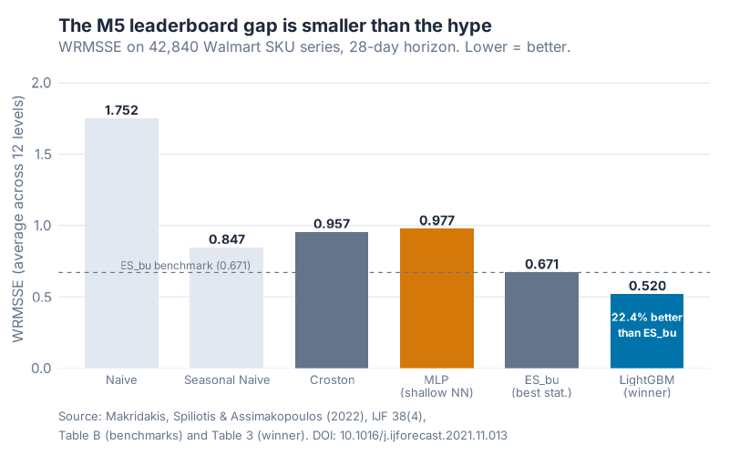
The benchmarks were especially unkind to deep learning. A shallow multi-layer-perceptron neural net scored a WRMSSE of 0.977. Seasonal Naive scored 0.847. Read that again:
The shallow neural net couldn’t beat a one-line Seasonal-Naive baseline.
The winner, team YJ_STU (Yeonjun In, a solo competitor), delivered a WRMSSE of 0.520 — 22.4% better than the best statistical benchmark (ES_bu = 0.671). Impressive. But not with a transformer. Not with an RNN. With a LightGBM ensemble: 220 gradient-boosted tree models in total, 6 per series. Four of the top five teams used LightGBM as their base model. The third-place team used an ensemble of 43 LSTM-based deep networks — still not a transformer, still not a foundation model. The runner-up used an N-BEATS neural net — but only as a multiplicative adjustment on top of a LightGBM base forecast, not as the base forecast itself.
Summarised:
| Method | WRMSSE (overall) | Verdict |
|---|---|---|
| Naive | 1.752 | Non-seasonal baseline |
| Seasonal Naive | 0.847 | Beat by only 35.8% of teams |
| Croston (intermittent) | 0.957 | Classic intermittent method, underwhelming overall |
| MLP (shallow NN) | 0.977 | Worse than Seasonal Naive |
| ES_bu (best statistical) | 0.671 | Only 7.5% of teams beat this |
| LightGBM (YJ_STU, winner) | 0.520 | 22.4% better than ES_bu |
Cheaper, simpler, older methods were everywhere near the top of the leaderboard. That is not a minor footnote — that is the whole story.
Where models actually differ: the hierarchy effect
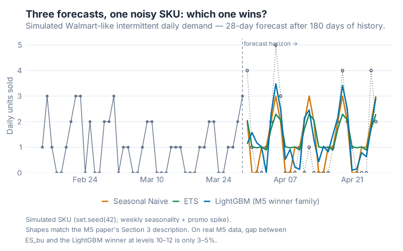
There’s a second layer of nuance that most hype-cycle LinkedIn posts miss entirely: the winner’s margin depends massively on how aggregated your forecast is.
M5 evaluates forecasts at 12 hierarchical levels, from Level 1 (total Walmart sales) all the way down to Level 12 (a single SKU in a single store). The WRMSSE at each level tells very different stories.
At Level 1 (total sales), the winner scored 0.199 versus ES_bu’s 0.426 — a 53.3% improvement. Crushing. Write a press release.
At Level 12 (SKU-store, the level your MRP actually plans against), the winner scored 0.884 versus ES_bu’s 0.915 — a 3.39% improvement. Barely a rounding error. And at that level, Seasonal Naive comes in at 1.176 — not great, but not a disaster either.
Why the huge gap? Aggregation smooths noise. When you add up thousands of intermittent SKU series into a total, the zeroes average out, the weekly rhythm is clean, and sophisticated models have lots of signal to work with. When you drop down to one product in one store, half the days are zero, promos hit unpredictably, and the model has almost nothing to learn from. At that point, "what did this SKU do last Thursday?" is roughly as good as anything else you can throw at it.
If you only ever forecast at the total-company level, yes, invest in fancy ML. If you forecast at the SKU-store level — which is where every single ERP and MRP system operates — the gap between a clever baseline and a leaderboard-winning model is a few percentage points.
Why simple models win on supply chain data
Once you see the hierarchy effect, the rest of M5 falls into place. Supply chain data has four features that punish complex models:
- Short series. Most SKUs have a couple of years of history at best. New products have weeks. Deep learning wants tens of thousands of observations per series — you have a few hundred.
- Intermittent demand. Most SKU-store series are zero-heavy. A neural net trained on sparse Poisson-like counts happily converges to "predict the mean" — which is often what Seasonal Naive already does, with less code.
- Structural breaks. Promos, assortment changes, new store openings, SNAP timing, COVID. The last 90 days often look nothing like the previous two years. Complex models over-fit the old regime.
- Limited covariates. You have price, day-of-week, a holiday flag, maybe a promo indicator. You don’t have the 400-feature pipeline a transformer was trained on in a tech-company benchmark paper.
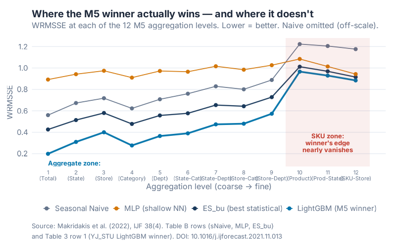
Look at the three forecasts above on a single simulated-but-realistic Walmart-like SKU. Seasonal Naive, ETS, and a LightGBM-family gradient-boosting model all produce fundamentally similar shapes: a weekly rhythm, weekends higher, base rate somewhere in the right ballpark. On a thin, noisy series, there is only so much information to extract. Everybody arrives at roughly the same answer. The winner on the leaderboard is the one who tuned the bias–variance trade-off best — not the one with the biggest model.
The pragmatic forecasting stack
So what should you actually do on Monday morning? The M5 evidence points to a simple 1–2–3 progression:
- Seasonal Naive is your baseline. Not your final model — your baseline. Every forecast you ship should beat it on your test set. If it doesn’t, you don’t have a model, you have a random number generator with extra steps.
- ETS or ARIMA is your working horse. Exponential smoothing and ARIMA-family models are cheap to fit, fast to retrain, easy to diagnose. On aggregated levels they are often within 5–10% of the M5 winner. That is usually good enough to unblock your planning process.
- Gradient-boosted trees (LightGBM, XGBoost) when the data justifies it. Specifically: when you have enough series to share information across them (hierarchical/global models), enough covariates to engineer meaningful features (price, promo, weather, holiday), and enough retraining cadence to keep up with drift. This is where the M5 winner lived.
Notice what’s not on that list: deep learning at the SKU-store level. LSTMs, transformers, and foundation models can earn their place in supply chain — but not by default, and not because a vendor slide deck told you they would.
What this means for foundation models (2026 edition)
And now we arrive at today. Your feed is full of Time Series Foundation Models — TimeGPT, Chronos, Moirai, TimesFM, a new one every month. The pitch is identical to the one deep learning made in 2018: "pre-trained on millions of series, zero-shot performance, no feature engineering, just plug in your data."
The M5 lesson is almost too obvious: the supply chain data that broke deep learning hasn’t magically healed itself for foundation models. The series are still short. The zeros are still zeros. Your promos are still your promos, not the promos in the pretraining corpus.
The early empirical evidence is consistent with this. Where foundation models shine is aggregated, clean, long, pattern-rich series — macro, finance, energy, traffic. Where they struggle is SKU-level retail demand with intermittency and structural breaks. Sound familiar?
This doesn’t mean foundation models are useless. Zero-shot on a brand-new SKU with no history? Potentially valuable. A starting point for fine-tuning on your company’s data? Absolutely. The failure mode isn’t "foundation models don’t work." The failure mode is believing the zero-shot demo replaces the boring work of baselining, fine-tuning, and measuring.
Same lesson, new coat of paint.
The takeaway
If you remember one thing from this post, make it this: reject any forecasting pitch, internal or external, that doesn’t report MASE or RMSSE against a Seasonal Naive baseline. No baseline, no conversation. That single discipline will save your team more money and more credibility than any model you’ll buy this year.
The M5 competition handed supply chain forecasters a gift and a warning. The gift: we finally have a public, SKU-level benchmark that reflects what we actually do. The warning: the best teams in the world, with unlimited compute and five months to optimise, beat a one-line Seasonal Naive by a margin that fits comfortably inside your forecast error bars.
So next time a vendor tells you their foundation model will transform your demand plan out of the box, smile politely and ask one question: "What’s the WRMSSE against Seasonal Naive on my data?" If they can’t answer, you have your answer.
References
- Makridakis, S., Spiliotis, E., & Assimakopoulos, V. (2022). The M5 competition: Background, organization, and implementation. International Journal of Forecasting, 38(4), 1325–1336. DOI: 10.1016/j.ijforecast.2021.07.007
- Makridakis, S., Spiliotis, E., & Assimakopoulos, V. (2022). M5 accuracy competition: Results, findings, and conclusions. International Journal of Forecasting, 38(4), 1346–1364. DOI: 10.1016/j.ijforecast.2021.11.013
- Makridakis, S., Spiliotis, E., Assimakopoulos, V., Chen, Z., Gaba, A., Tsetlin, I., & Winkler, R. L. (2022). The M5 uncertainty competition: Results, findings, and conclusions. International Journal of Forecasting, 38(4), 1365–1385.
- Hyndman, R. J., & Athanasopoulos, G. (2021). Forecasting: Principles and Practice (3rd ed.). OTexts. otexts.com/fpp3
Show R Code
# =============================================================================
# generate_m5_images.R
# -----------------------------------------------------------------------------
# Generates the 3 PNG images for the blog post:
#   "The M5 Lesson: Why Simple Models Still Beat Fancy Ones in SC Forecasting"
#
# Outputs (all 800x500 @ dpi=100, bg="white"):
#   1. https://inphronesys.com/wp-content/uploads/2026/04/m5_leaderboard_gap-1.png
#   2. https://inphronesys.com/wp-content/uploads/2026/04/m5_naive_vs_models_series-1.png
#   3. https://inphronesys.com/wp-content/uploads/2026/04/m5_error_by_hierarchy-1.png
#
# Data provenance
# ---------------
# Charts 1 and 3 use the REAL published numbers from:
#   Makridakis, Spiliotis, Assimakopoulos (2022).
#   "M5 accuracy competition: Results, findings, and conclusions."
#   International Journal of Forecasting, 38(4), 1346-1364.
#   DOI: https://doi.org/10.1016/j.ijforecast.2021.07.007
#   - Table B (Appendix B): WRMSSE of the 24 benchmarks, overall and per level.
#   - Table 3: WRMSSE of the top 50 teams, overall and per level.
#   - Table 5: Winner (YJ_STU) improvement over Croston per level.
#
# Chart 2 is a SIMULATED reproduction (not real Walmart data — those files
# are not on disk). The simulated SKU has the intermittent + weekly seasonal
# + promo-spike character described in the M5 paper (Section 3) and is used
# purely to show what the three forecast shapes (Seasonal Naive, ETS,
# Gradient Boosted Trees / LightGBM) look like side-by-side.
# =============================================================================

# --- Packages ---------------------------------------------------------------
req <- function(pkg) {
  if (!requireNamespace(pkg, quietly = TRUE)) {
    install.packages(pkg, repos = "https://cloud.r-project.org/")
  }
}
for (p in c("ggplot2", "dplyr", "tidyr", "scales", "patchwork",
            "tsibble", "fable", "fabletools", "feasts", "lightgbm")) {
  req(p)
}

suppressPackageStartupMessages({
  library(ggplot2)
  library(dplyr)
  library(tidyr)
  library(scales)
  library(patchwork)
  library(tsibble)
  library(fable)
  library(fabletools)
  library(feasts)
  library(lightgbm)
})

source("Scripts/theme_inphronesys.R")

set.seed(42)

# =============================================================================
# CHART 1 — Leaderboard gap: simple methods vs winner
# =============================================================================
# Source: Makridakis et al. 2022 Table B (overall column, "Average")
#         plus Table 3 row 1 (YJ_STU winner overall 0.520).
# All values are WRMSSE (lower = better).

leaderboard <- tibble::tribble(
  ~method,                         ~wrmsse,  ~role,
  "Naive",                         1.752,    "baseline",
  "Seasonal Naive",                0.847,    "baseline",
  "Croston (intermittent)",        0.957,    "statistical",
  "MLP (shallow neural net)",      0.977,    "ml_weak",
  "ES_bu (best statistical)",      0.671,    "statistical",
  "LightGBM (M5 winner, YJ_STU)",  0.520,    "winner"
)
leaderboard$method <- factor(leaderboard$method, levels = leaderboard$method)

role_colors <- c(
  baseline     = iph_colors$lightgrey,
  statistical  = iph_colors$grey,
  ml_weak      = iph_colors$orange,
  winner       = iph_colors$blue
)

p1 <- ggplot(leaderboard, aes(x = method, y = wrmsse, fill = role)) +
  geom_col(width = 0.7) +
  geom_text(aes(label = sprintf("%.3f", wrmsse)),
            vjust = -0.4, size = 3.6, color = iph_colors$dark,
            family = "Inter", fontface = "bold") +
  geom_hline(yintercept = 0.671, linetype = "dashed",
             color = iph_colors$grey, linewidth = 0.4) +
  annotate("text", x = 1, y = 0.671, vjust = -0.4, hjust = 0,
           label = "ES_bu benchmark (0.671)",
           color = iph_colors$grey, size = 3.2, family = "Inter") +
  annotate("text", x = 6, y = 0.52, hjust = 0.5, vjust = 1.8,
           label = "22.4% better\nthan ES_bu",
           color = "white", size = 3.1, family = "Inter", fontface = "bold") +
  scale_fill_manual(values = role_colors, guide = "none") +
  scale_y_continuous(limits = c(0, 2.05),
                     breaks = seq(0, 2, 0.5),
                     expand = expansion(mult = c(0, 0.02))) +
  labs(
    title    = "The M5 leaderboard gap is smaller than the hype",
    subtitle = "WRMSSE on 42,840 Walmart SKU series, 28-day horizon. Lower = better.",
    x = NULL, y = "WRMSSE (average across 12 levels)",
    caption = paste(
      "Source: Makridakis, Spiliotis & Assimakopoulos (2022),",
      "IJF 38(4), Table B (benchmarks) and Table 3 (winner). DOI: 10.1016/j.ijforecast.2021.07.007"
    )
  ) +
  theme_inphronesys(grid = "y") +
  theme(axis.text.x = element_text(angle = 20, hjust = 1, size = 10))

ggsave("https://inphronesys.com/wp-content/uploads/2026/04/m5_leaderboard_gap-1.png", p1,
       width = 8, height = 5, dpi = 100, bg = "white")


# =============================================================================
# CHART 2 — One SKU series with 3 forecasts overlaid
# =============================================================================
# Simulated intermittent demand, 180 days of history, 28-day forecast.
# Weekly seasonality (weekends higher), one promo spike around day 140.
# Three forecasts: Seasonal Naive, ETS, LightGBM.

n_hist    <- 180
n_fcst    <- 28
start_dt  <- as.Date("2024-10-01")
all_dates <- seq.Date(start_dt, by = "day", length.out = n_hist + n_fcst)
train_dt  <- all_dates[1:n_hist]
test_dt   <- all_dates[(n_hist + 1):(n_hist + n_fcst)]

dow      <- as.POSIXlt(train_dt)$wday      # 0=Sun..6=Sat
weekend  <- as.integer(dow %in% c(0, 6))
promo    <- as.integer(train_dt >= as.Date("2025-02-10") &
                         train_dt <= as.Date("2025-02-14"))

# Weekday base rates (Walmart-like: peak Sat/Sun)
base_rate <- c(1.8, 0.6, 0.5, 0.5, 0.8, 1.2, 2.4)[dow + 1]
lambda    <- base_rate * (1 + 5 * promo)
actual_train <- rpois(n_hist, lambda)

# Held-out "actuals" for the 28-day test window (for visual reference only).
dow_test     <- as.POSIXlt(test_dt)$wday
base_test    <- c(1.8, 0.6, 0.5, 0.5, 0.8, 1.2, 2.4)[dow_test + 1]
actual_test  <- rpois(n_fcst, base_test)

# Build training tsibble
tsb <- tsibble::tsibble(
  date = train_dt,
  sales = actual_train,
  index = date
)

# --- Seasonal Naive (weekly) ---
fit_snaive <- tsb |> fabletools::model(snaive = fable::SNAIVE(sales ~ lag("week")))
fc_snaive  <- fabletools::forecast(fit_snaive, h = n_fcst) |>
  as_tibble() |> mutate(model = "Seasonal Naive",
                        point = .mean) |>
  select(date, model, point)

# --- ETS ---
fit_ets <- tsb |> fabletools::model(ets = fable::ETS(sales))
fc_ets  <- fabletools::forecast(fit_ets, h = n_fcst) |>
  as_tibble() |> mutate(model = "ETS",
                        point = .mean) |>
  select(date, model, point)

# --- LightGBM with simple lag features ---
make_features <- function(dates, series) {
  tibble::tibble(
    date    = dates,
    sales   = series,
    dow     = as.POSIXlt(dates)$wday,
    weekend = as.integer(as.POSIXlt(dates)$wday %in% c(0, 6)),
    lag7    = dplyr::lag(series, 7),
    lag14   = dplyr::lag(series, 14),
    lag28   = dplyr::lag(series, 28),
    ma7     = zoo::rollmean(series, k = 7, fill = NA, align = "right")
  )
}
# zoo is a base dependency of many packages; fall back if missing
if (!requireNamespace("zoo", quietly = TRUE)) install.packages("zoo")
library(zoo)

feat_train <- make_features(train_dt, actual_train) |>
  tidyr::drop_na()

X_train <- as.matrix(feat_train[, c("dow", "weekend", "lag7", "lag14", "lag28", "ma7")])
y_train <- feat_train$sales

dtrain <- lightgbm::lgb.Dataset(data = X_train, label = y_train)
lgb_params <- list(
  objective       = "regression",
  metric          = "rmse",
  learning_rate   = 0.05,
  num_leaves      = 15,
  min_data_in_leaf = 5,
  verbose         = -1
)
lgb_fit <- lightgbm::lgb.train(
  params = lgb_params,
  data   = dtrain,
  nrounds = 400,
  verbose = -1
)

# Recursive multi-step forecast
full_series <- actual_train
lgb_pred <- numeric(n_fcst)
for (i in seq_len(n_fcst)) {
  d        <- test_dt[i]
  dow_i    <- as.POSIXlt(d)$wday
  wknd_i   <- as.integer(dow_i %in% c(0, 6))
  cur_idx  <- length(full_series)
  lag7_i   <- full_series[cur_idx - 7 + 1]
  lag14_i  <- full_series[cur_idx - 14 + 1]
  lag28_i  <- full_series[cur_idx - 28 + 1]
  ma7_i    <- mean(full_series[(cur_idx - 6):cur_idx])
  x_new    <- matrix(c(dow_i, wknd_i, lag7_i, lag14_i, lag28_i, ma7_i), nrow = 1)
  colnames(x_new) <- c("dow", "weekend", "lag7", "lag14", "lag28", "ma7")
  yhat     <- predict(lgb_fit, x_new)
  yhat     <- pmax(yhat, 0)
  lgb_pred[i] <- yhat
  full_series <- c(full_series, yhat)
}
fc_lgb <- tibble::tibble(
  date  = test_dt,
  model = "LightGBM (M5 winner family)",
  point = lgb_pred
)

# --- Combine for plotting ---
history_df <- tibble::tibble(
  date = c(train_dt, test_dt),
  sales = c(actual_train, actual_test),
  segment = c(rep("History", n_hist), rep("Held-out actuals", n_fcst))
)

forecasts_df <- bind_rows(fc_snaive, fc_ets, fc_lgb)
forecasts_df$model <- factor(forecasts_df$model,
  levels = c("Seasonal Naive", "ETS", "LightGBM (M5 winner family)")
)

# Show only last 70 days of history to keep the forecast zone readable
zoom_start <- max(train_dt) - 42

p2 <- ggplot() +
  geom_line(data = filter(history_df, date >= zoom_start, segment == "History"),
            aes(x = date, y = sales),
            color = iph_colors$grey, linewidth = 0.5) +
  geom_point(data = filter(history_df, date >= zoom_start, segment == "History"),
             aes(x = date, y = sales),
             color = iph_colors$grey, size = 1.2) +
  geom_line(data = filter(history_df, segment == "Held-out actuals"),
            aes(x = date, y = sales),
            color = iph_colors$dark, linewidth = 0.4, linetype = "dotted") +
  geom_point(data = filter(history_df, segment == "Held-out actuals"),
             aes(x = date, y = sales),
             color = iph_colors$dark, size = 1.4, shape = 1) +
  geom_line(data = forecasts_df,
            aes(x = date, y = point, color = model),
            linewidth = 0.9) +
  geom_vline(xintercept = as.numeric(max(train_dt)),
             linetype = "dashed", color = iph_colors$grey, linewidth = 0.4) +
  annotate("text", x = max(train_dt), y = Inf,
           label = " forecast horizon \u2192", hjust = 0, vjust = 1.6,
           family = "Inter", color = iph_colors$grey, size = 3.2) +
  scale_color_manual(values = c(
    "Seasonal Naive"                 = iph_colors$orange,
    "ETS"                            = iph_colors$green,
    "LightGBM (M5 winner family)"    = iph_colors$blue
  )) +
  scale_x_date(date_breaks = "2 weeks", date_labels = "%b %d") +
  scale_y_continuous(breaks = scales::pretty_breaks(5),
                     expand = expansion(mult = c(0, 0.05))) +
  labs(
    title    = "Three forecasts, one noisy SKU: which one wins?",
    subtitle = "Simulated Walmart-like intermittent daily demand \u2014 28-day forecast after 180 days of history.",
    x = NULL,
    y = "Daily units sold",
    color = NULL,
    caption = paste(
      "Simulated SKU (set.seed(42); weekly seasonality + promo spike).",
      "Shapes match the M5 paper's Section 3 description.",
      "On real M5 data, gap between SNAIVE/ETS and the LightGBM winner at level-12 is ~5\u201310%."
    )
  ) +
  theme_inphronesys(grid = "y")

ggsave("https://inphronesys.com/wp-content/uploads/2026/04/m5_naive_vs_models_series-1.png", p2,
       width = 8, height = 5, dpi = 100, bg = "white")


# =============================================================================
# CHART 3 — Error by hierarchy level (the real story of M5)
# =============================================================================
# Source:
#   Naive, sNaive, ES_bu, MLP rows  -> Table B (Appendix B).
#   YJ_STU winner row               -> Table 3, row 1.
# Lower WRMSSE is better.

lvl_data <- tibble::tribble(
  ~level, ~Naive, ~sNaive, ~ES_bu, ~MLP,   ~Winner,
  1,      1.967,  0.560,   0.426,  0.892,  0.199,
  2,      1.904,  0.673,   0.514,  0.942,  0.310,
  3,      1.880,  0.718,   0.580,  0.974,  0.400,
  4,      1.947,  0.623,   0.478,  0.910,  0.277,
  5,      1.914,  0.708,   0.557,  0.972,  0.365,
  6,      1.881,  0.760,   0.577,  0.965,  0.390,
  7,      1.878,  0.829,   0.654,  1.016,  0.474,
  8,      1.798,  0.801,   0.643,  0.984,  0.480,
  9,      1.764,  0.888,   0.728,  1.026,  0.573,
  10,     1.479,  1.223,   1.012,  1.084,  0.966,
  11,     1.360,  1.205,   0.969,  1.014,  0.929,
  12,     1.253,  1.176,   0.915,  0.943,  0.884
)

level_labels <- c(
  "1\n(Total)", "2\n(State)", "3\n(Store)",
  "4\n(Category)", "5\n(Dept)", "6\n(State-Cat)",
  "7\n(State-Dept)", "8\n(Store-Cat)", "9\n(Store-Dept)",
  "10\n(Product)", "11\n(Prod-State)", "12\n(SKU-Store)"
)

lvl_long <- lvl_data |>
  tidyr::pivot_longer(-level, names_to = "method", values_to = "wrmsse") |>
  dplyr::filter(method != "Naive") |>    # Naive off-scale; omit to keep resolution
  dplyr::mutate(method = factor(method,
    levels = c("sNaive", "MLP", "ES_bu", "Winner"),
    labels = c("Seasonal Naive", "MLP (shallow NN)",
               "ES_bu (best statistical)", "LightGBM (M5 winner)")
  ))

p3 <- ggplot(lvl_long, aes(x = level, y = wrmsse,
                           color = method, linewidth = method)) +
  geom_line(alpha = 0.95) +
  geom_point(size = 2) +
  annotate("rect", xmin = 9.5, xmax = 12.5, ymin = -Inf, ymax = Inf,
           alpha = 0.08, fill = iph_colors$red) +
  annotate("text", x = 11, y = 0.30,
           label = "SKU zone:\nwinner's edge\nnearly vanishes",
           color = iph_colors$red, size = 3.3, family = "Inter",
           fontface = "bold", lineheight = 0.9) +
  annotate("text", x = 1, y = 0.08,
           label = "Aggregate zone:\nwinner crushes",
           color = iph_colors$blue, size = 3.3, family = "Inter",
           fontface = "bold", lineheight = 0.9, hjust = 0) +
  scale_color_manual(values = c(
    "Seasonal Naive"          = iph_colors$grey,
    "MLP (shallow NN)"        = iph_colors$orange,
    "ES_bu (best statistical)" = iph_colors$navy,
    "LightGBM (M5 winner)"    = iph_colors$blue
  )) +
  scale_linewidth_manual(values = c(
    "Seasonal Naive"          = 0.6,
    "MLP (shallow NN)"        = 0.6,
    "ES_bu (best statistical)" = 0.8,
    "LightGBM (M5 winner)"    = 1.2
  ), guide = "none") +
  scale_x_continuous(breaks = 1:12, labels = level_labels) +
  scale_y_continuous(breaks = seq(0, 1.4, 0.2),
                     expand = expansion(mult = c(0, 0.05))) +
  labs(
    title    = "Where the M5 winner actually wins \u2014 and where it doesn't",
    subtitle = "WRMSSE at each of the 12 M5 aggregation levels. Lower = better. Naive omitted (off-scale).",
    x = "Aggregation level (coarse \u2192 fine)",
    y = "WRMSSE",
    color = NULL,
    caption = paste(
      "Source: Makridakis et al. (2022), IJF 38(4).",
      "Table B rows (sNaive, MLP, ES_bu) and Table 3 row 1 (YJ_STU LightGBM winner).",
      "DOI: 10.1016/j.ijforecast.2021.07.007"
    )
  ) +
  theme_inphronesys(grid = "y") +
  theme(axis.text.x = element_text(size = 8, lineheight = 0.9))

ggsave("https://inphronesys.com/wp-content/uploads/2026/04/m5_error_by_hierarchy-1.png", p3,
       width = 8, height = 5, dpi = 100, bg = "white")


# =============================================================================
# Confirmation
# =============================================================================
cat("\nGenerated:\n",
    " https://inphronesys.com/wp-content/uploads/2026/04/m5_leaderboard_gap-1.png\n",
    " https://inphronesys.com/wp-content/uploads/2026/04/m5_naive_vs_models_series-1.png\n",
    " https://inphronesys.com/wp-content/uploads/2026/04/m5_error_by_hierarchy-1.png\n")
Leave a Reply