Picture a sticky note stuck to a monitor. It reads: „Same as last year.“ That sticky note is a forecast. It cost nothing, took two seconds, and required zero meetings.
Now picture your demand planning process. A statistical engine. An analyst who knows the accounts. A monthly S&OP meeting where five smart people argue about the number. All of it expensive. All of it slow.
Here’s the question. Does any of that beat the sticky note?
A lot of the time, no. That’s the whole story of Forecast Value Added, and it’s why I think FVA is the single most useful metric most demand planners have never run.
What FVA actually is (and why it stings)
Forecast Value Added is borrowed straight from medicine. In a drug trial, you don’t ask „did the patient get better?“ You ask „did they get better than the ones who took the sugar pill?“ The placebo is the benchmark. The drug only earns its license if it beats the placebo.
FVA does the same thing to forecasting. The placebo is the naive forecast: the dumbest possible guess, like „next month equals the same month last year.“ Every fancier step in your process (the model, the analyst, the executive review) is a treatment. A treatment only earns its keep if it beats the placebo.
Michael Gilliland built this idea into a standard metric in The Business Forecasting Deal (2010). The genius of it is the cruelty. FVA doesn’t care how sophisticated your model is. It doesn’t care how senior the person tweaking the number is. It asks one thing: are you adding accuracy, or just adding cost?
Most forecasting processes have never been asked that question. When they are, the answer is often embarrassing.
Why the naive forecast is such a brutal benchmark
People underestimate the sticky note. They shouldn’t.
„Same month last year“ already carries your seasonality for free. Sell more ice cream in July? The naive forecast knows, because last July is right there in the data. No model to fit, no parameters to tune, no overfitting. It’s free, fast, and surprisingly hard to beat.
That’s the trap. A bad model can lose to it. So can a good model that’s been „improved“ by too many hands. The benchmark doesn’t move, doesn’t get tired, and doesn’t have a quarterly target to hit. It just sits there, quietly outperforming.
If your million-euro planning stack can’t beat a sticky note, that’s not a small problem. That’s the problem.
The four-step process we put on trial
To show this in action, I ran a simulation. (Realistic numbers, not a real company. Synthetic monthly demand for a mid-size manufacturer’s 50-SKU portfolio, four years of data, scored on a 12-month holdout.) The full R code is at the bottom if you want to reproduce every figure.
The process has four steps, which is how most real demand plans actually work:
- Naive (the placebo): seasonal naive, same month last year.
- Statistical: a proper model (STL decomposition plus ETS) fit on three years of history.
- Analyst override: a demand planner nudges the numbers based on judgment.
- Executive / consensus: the S&OP meeting produces the final, signed-off forecast.
Each step gets scored with MAPE (mean absolute percentage error). Lower is better. Then we measure how much accuracy each step added or destroyed versus the step before it. That’s the FVA.
I’ll be honest: I expected the model to add value and the humans to add a little more. I was half right.
The stairstep: the forecast got better, then the humans got hold of it
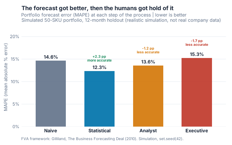
Watch the shape. The error drops when the model takes over, then climbs right back up as the humans get involved. Down the stairs, then back up. The final number ends up higher than where we started.
Here’s the canonical FVA stairstep report, the table every demand planning team should be able to produce on demand:
| Process step | MAPE | FVA vs naive | FVA vs previous step |
|---|---|---|---|
| Naive | 14.6% | 0.0 pp | n/a (benchmark) |
| Statistical | 12.3% | +2.3 pp | +2.3 pp |
| Analyst | 13.6% | +1.1 pp | −1.2 pp |
| Executive (final) | 15.3% | −0.6 pp | −1.7 pp |
Read the last column slowly. The statistical model cut error by 2.3 points versus the naive benchmark. Good model. Worth its license.
Then the analyst override gave back 1.2 of those points. Then the executive consensus gave back another 1.7. The two human steps combined destroyed 2.9 points of accuracy. The model added 2.3. Do the arithmetic.
The final, signed-off, everyone-agreed-on-it forecast lands at 15.3% MAPE. The sticky note sits at 14.6%. The entire expensive process ended up worse than doing nothing. Net FVA of the whole machine: −0.6 percentage points.
That’s not a typo. The consensus forecast lost to the placebo.
The waterfall: where the value leaks out
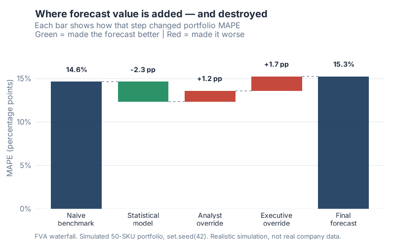
The waterfall makes the leak impossible to miss. One green bar (the model) pulling error down. Two red bars (analyst, then executive) shoving it back up, past the starting line.
Why does this happen? The simulation models two failure modes that show up constantly in real planning:
The analyst override is mostly noise. Small judgmental tweaks that feel like insight but average out to nothing useful. This isn’t me being cynical about planners. The research backs it up, and I’ll get to that evidence in a minute.
The executive consensus is worse, and worse on purpose. It carries optimism bias: a systematic upward inflation, because the forecast quietly becomes a target. Sales wants headroom. Leadership wants growth on the slide. So the number creeps up, regardless of what demand is actually doing. Bias, unlike noise, doesn’t average out. It just accumulates.
How often does each step actually beat naive?
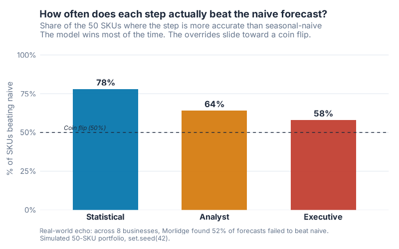
Portfolio averages can hide things, so here’s a different cut: on how many of the 50 SKUs does each step actually beat the naive forecast?
The statistical model wins on 78% of SKUs. (It still loses to naive on the other 22%, which tells you how genuinely tough that benchmark is, even for a good model.) The analyst override slides to 64%. The executive consensus drops to 58%, drifting toward the 50% coin-flip line.
Each human touch nudges the process closer to „we’d have done about as well flipping a coin.“ That’s the trend that should keep a planning lead up at night.
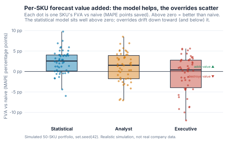
Look at the spread per SKU and the same story holds. The model’s dots sit comfortably above the zero line. The override dots scatter downward, plenty of them dipping below zero into value-destroyed territory.
This isn’t just my simulation
I built a toy world to make the mechanism visible. But the pattern is real, and it’s documented.
Steve Morlidge studied forecasts across eight consumer and industrial businesses. The finding, reported in the peer-reviewed survey by Petropoulos et al. (2022): 52% of those forecasts failed to beat a naive forecast. More than half. In real companies. With real planning teams.
(Quick note so nobody conflates the two numbers: my simulation says 42% of final forecasts failed to beat naive. Morlidge’s real-world figure is 52% of forecasts overall. Different studies, same direction, both ugly.)
And the override damage isn’t speculation either. Fildes, Goodwin, Lawrence and Nikolopoulos (2009) evaluated more than 60,000 forecasts from four supply-chain companies. Small judgmental adjustments usually hurt. Large downward ones usually helped. Upward ones, the kind a growth-hungry S&OP meeting loves, rarely helped at all.
The data has been telling us this since 2009. Most teams just never measured it on their own numbers.
How to run FVA yourself: the Monday-morning roadmap
You don’t need a software license or a data science team. You need a spreadsheet and the discipline to keep score. Here’s the process, start to finish.
1. Map your process steps. Write down every stage where the forecast changes hands. Statistical engine, demand planner, regional override, S&OP consensus, whatever yours looks like. Each handoff is a step you’ll score.
2. Pick your naive benchmark. For seasonal products, use seasonal naive (same period last year). For flat or slow movers, use the last actual carried forward (random-walk naive). Pick one, write it down, don’t change it midstream.
3. Capture the forecast at every step. This is the part most teams skip, and without it FVA is impossible. Freeze and store the number as it leaves each stage. The model’s raw output before the planner touches it. The planner’s number before the meeting. The final consensus. Same forecast horizon for all of them.
4. Wait for actuals, then score MAPE per step. Once the real demand lands, compute MAPE for each captured forecast against the actuals, per SKU, then average across the portfolio. Same months, same items, apples to apples.
5. Build the stairstep report. Lay the steps in a table like the one above. Two FVA columns: versus naive, and versus the previous step. The second column is where the bodies are buried. It shows you exactly which handoff added accuracy and which one torched it.
6. Act on it. Kill the steps that destroy value. This is the point of the whole exercise, and it takes a spine. If the analyst override has negative FVA for three cycles running, stop overriding by default. If the executive layer only inflates, take it out of the accuracy chain and call it what it is: a business target, not a forecast. Keep the steps with positive FVA. Retire or redesign the rest.
That last step is where FVA earns its reputation as a politically dangerous metric. You’re about to prove, with numbers, that someone senior makes the forecast worse. Bring the chart, not the accusation.
Your one-afternoon proof of concept
The roadmap above is the full program. Here’s the stripped-down version you can finish before lunch, on a single product family, to find out whether any of this even applies to you:
- Pull one family’s actuals plus the final forecasts you already saved, last six months. Nothing fancy. One sheet.
- Add one column: seasonal naive, this month equals the same month last year. That’s your placebo.
- Compare MAPE: your final forecast versus naive. Lose to the sticky note and you’ve got your headline and your business case in a single chart. That’s your cue to go run the full six-step stairstep above.
The sticky note is on the wall. Go find out if your process beats it.
Interactive Dashboard
Want to see how the stairstep moves when you change the assumptions? Push the model’s skill up, dial the analyst noise and executive optimism up or down, and watch the FVA recompute live.
Interactive Dashboard
Explore the data yourself — adjust parameters and see the results update in real time.
Show R Code
# =============================================================================
# generate_fva_images.R
# FVA asks a brutally simple question (Gilliland, "The Business Forecasting
# Deal", 2010): does each step of the forecasting process beat a dirt-simple
# naive forecast, or is it expensive theater? The naive forecast is the
# placebo; the statistical model and the human overrides are treatments.
# A treatment only earns its keep if it beats the placebo.
#
# This script builds a REALISTIC SIMULATION (not real company data) of a
# mid-size manufacturer's 50-SKU portfolio over 48 months, runs a four-step
# forecasting process, and computes the canonical FVA "stairstep" report.
# Run from the project root:  Rscript Scripts/generate_fva_images.R
# =============================================================================

source("Scripts/theme_inphronesys.R")

suppressPackageStartupMessages({
  library(ggplot2)
  library(dplyr)
  library(tidyr)
  library(scales)
  library(forecast)   # stlf() / ets() — genuine exponential smoothing
})

set.seed(42)

# ---- 1. Simulate a realistic demand-planning scenario -----------------------
# 50 SKUs, 48 monthly periods. First 36 months = history used to fit/benchmark;
# last 12 months = evaluation holdout. Demand = level + trend + seasonality + noise.
n_sku    <- 50
n_months <- 48
train_n  <- 36
horizon  <- n_months - train_n

season_shape <- c(0.86, 0.82, 0.94, 1.04, 1.12, 1.18,
                  1.20, 1.14, 1.05, 0.98, 0.90, 1.08)

sku_panel <- list()
for (s in seq_len(n_sku)) {
  level    <- runif(1, 250, 2000)
  trend    <- rnorm(1, mean = level * 0.005, sd = level * 0.004)
  amp      <- runif(1, 0.75, 1.30)
  season   <- 1 + (season_shape - 1) * amp
  noise_sd <- runif(1, 0.09, 0.16)

  demand <- numeric(n_months)
  for (t in seq_len(n_months)) {
    base_t <- level + trend * (t - 1)
    sfac   <- season[((t - 1) %% 12) + 1]
    shock  <- exp(rnorm(1, 0, noise_sd))
    demand[t] <- max(round(base_t * sfac * shock), 1)
  }
  sku_panel[[s]] <- data.frame(sku = s, month = seq_len(n_months), demand = demand)
}
panel <- bind_rows(sku_panel)

# ---- 2. Build the four-step forecasting process -----------------------------
#   STEP 1  Naive       — seasonal naive: same month last year.
#   STEP 2  Statistical — STL + ETS on the 36-month history (genuinely adds value).
#   STEP 3  Analyst     — small, ~zero-mean judgmental nudges (mostly noise).
#   STEP 4  Executive   — S&OP optimism bias: systematic upward inflation.
ets_models <- character(0)
rows <- list()

for (s in seq_len(n_sku)) {
  d        <- panel$demand[panel$sku == s]
  train    <- d[1:train_n]
  test_idx <- (train_n + 1):n_months
  actual   <- d[test_idx]

  f_naive <- d[test_idx - 12]                 # seasonal naive
  f_rw    <- rep(train[train_n], horizon)     # random-walk naive (secondary)

  ts_train <- ts(train, frequency = 12)
  fit      <- stlf(ts_train, h = horizon, method = "ets")
  ets_models <- c(ets_models, fit$model$method)
  f_stat   <- pmax(as.numeric(fit$mean), 1)

  big_mover   <- runif(1) < 0.25
  adj_sd      <- if (big_mover) 0.10 else 0.04
  analyst_adj <- rnorm(horizon, mean = 0, sd = adj_sd)
  f_analyst   <- pmax(f_stat * (1 + analyst_adj), 1)

  exec_bias <- rnorm(horizon, mean = 0.075, sd = 0.04)
  f_exec    <- pmax(f_analyst * (1 + exec_bias), 1)

  rows[[s]] <- data.frame(
    sku = s, month = test_idx, actual = actual,
    Naive = f_naive, Statistical = f_stat,
    Analyst = f_analyst, Executive = f_exec, rw = f_rw
  )
}
fc <- bind_rows(rows)

# ---- 3. Accuracy metrics — MAPE per SKU per step, averaged over portfolio ----
ape <- function(actual, forecast) abs(actual - forecast) / actual * 100
step_levels <- c("Naive", "Statistical", "Analyst", "Executive")

sku_mape <- fc %>%
  group_by(sku) %>%
  summarise(
    Naive       = mean(ape(actual, Naive)),
    Statistical = mean(ape(actual, Statistical)),
    Analyst     = mean(ape(actual, Analyst)),
    Executive   = mean(ape(actual, Executive)),
    rw          = mean(ape(actual, rw)),
    .groups = "drop"
  )

portfolio <- sku_mape %>%
  summarise(across(c(Naive, Statistical, Analyst, Executive, rw), mean))

mape_naive <- portfolio$Naive   # 14.6%
mape_stat  <- portfolio$Statistical  # 12.3%
mape_anal  <- portfolio$Analyst      # 13.6%
mape_exec  <- portfolio$Executive    # 15.3%

# Stairstep report: FVA vs naive and FVA vs previous step
stair <- data.frame(step = factor(step_levels, levels = step_levels),
                    mape = c(mape_naive, mape_stat, mape_anal, mape_exec))
stair$fva_vs_naive <- mape_naive - stair$mape
stair$fva_vs_prev  <- c(NA, -diff(stair$mape))

# % of SKUs where each step beats the naive benchmark
beat <- sku_mape %>%
  summarise(
    Statistical = mean(Statistical < Naive) * 100,   # 78%
    Analyst     = mean(Analyst     < Naive) * 100,   # 64%
    Executive   = mean(Executive   < Naive) * 100    # 58%
  )

# Per-SKU FVA vs naive for the distribution chart
sku_fva <- sku_mape %>%
  transmute(sku,
            Statistical = Naive - Statistical,
            Analyst     = Naive - Analyst,
            Executive   = Naive - Executive) %>%
  pivot_longer(-sku, names_to = "step", values_to = "fva") %>%
  mutate(step = factor(step, levels = c("Statistical", "Analyst", "Executive")))

# ---- 4. Charts (theme_inphronesys, 800x500, white bg) -----------------------
step_cols <- c("Naive" = iph_colors$grey, "Statistical" = iph_colors$blue,
               "Analyst" = iph_colors$orange, "Executive" = iph_colors$red)

# CHART 1: stairstep — MAPE by process step
ggplot(stair, aes(step, mape, fill = step)) +
  geom_col(width = 0.62, alpha = 0.92) +
  geom_text(aes(label = sprintf("%.1f%%", mape)), vjust = -0.6,
            family = "Inter", fontface = "bold", size = 4.2) +
  scale_fill_manual(values = step_cols, guide = "none") +
  labs(title = "The forecast got better, then the humans got hold of it",
       x = NULL, y = "MAPE (mean absolute % error)") +
  theme_inphronesys(base_size = 13, grid = "y")
ggsave("https://inphronesys.com/wp-content/uploads/2026/06/fva_stairstep.png", width = 8, height = 5, dpi = 100, bg = "white")

# CHART 2 waterfall, CHART 3 % beat naive, CHART 4 per-SKU distribution
# (full plotting code in Scripts/generate_fva_images.R)
References
- Gilliland, M. (2010). The Business Forecasting Deal: Exposing Myths, Eliminating Bad Practices, Providing Practical Solutions. Hoboken, NJ: John Wiley & Sons (Wiley & SAS Business Series). ISBN 978-0-470-57443-0. Publisher page
- Gilliland, M. (SAS Institute). „Forecast Value Added Analysis: Step-by-Step.“ SAS white paper (PDF)
- Morlidge, S. (2013). „How Good Is a ‚Good‘ Forecast? Forecast Errors and Their Avoidability,“ Foresight: The International Journal of Applied Forecasting, Issue 30. The „52% of forecasts across eight businesses failed to beat naive“ figure is reported in Petropoulos, F., et al. (2022), „Forecasting: theory and practice,“ International Journal of Forecasting. Open version (PDF)
- Fildes, R., Goodwin, P., Lawrence, M., & Nikolopoulos, K. (2009). „Effective forecasting and judgmental adjustments: an empirical evaluation and strategies for improvement in supply-chain planning,“ International Journal of Forecasting, 25(1), 3–23. ScienceDirect
Schreibe einen Kommentar