
A plant runs for thirty days. Every machine but one reports 100% utilisation, and the exception is the one nobody watches. The shared parts shelf never ends a day empty and never ends one below 60 units, so the daily inventory report is clean all month. Nobody ordered more than usual. And one of the two customers receives 57% of what they ordered.
Nothing broke. No supplier missed, no machine went down, no demand spike arrived. The plant made the wrong thing first, and in that shape of plant, wrong is close to permanent.
Every factory simulation ever built teaches you the same lesson: find the slowest resource, that sets your pace. True, and only half the story. The bottleneck’s speed tells you how much you can make. The bottleneck’s position in the topology tells you who goes short when you make the wrong thing. Those are two different questions, and the second one has an answer that almost nobody outside an APICS study group can name.
It’s called VATI.
What VATI actually is
Take one product family. Draw its routing on paper: raw material at the bottom, finished goods at the top, a dot for every operation and a line for every material move. Then step back and squint at the silhouette.
You get one of four letters.
I is a straight line. One route, one sequence, one obvious slow station. A bottling line, a dedicated single-product assembly line.
V is one trunk fanning out. Few raw materials in, many finished SKUs out. Steel, oil refining, paper, dairy, textiles.
A is many legs converging. Distinct raw materials run up separate fabrication legs, meet at subassemblies, and meet again at one final assembly. Aerospace, shipbuilding, heavy equipment.
T is both, stacked. Legs converge into a pool of common parts, and those parts then fan out into many finished configurations. Configure-to-order electronics is the textbook case.
VAT analysis grew out of Eliyahu Goldratt’s Theory of Constraints work, and the APICS Dictionary carries entries for all three letters. The fourth one is softer ground. The I is commonly described as a later practitioner addition, and just as commonly described as a V-plant that hasn’t reached its split yet rather than a genuine fourth category. I’ve kept it in this post because it’s the control group. It’s the only shape where your intuition about bottlenecks is fully correct, which is exactly what makes the other three interesting.
Two things VATI is not. It’s not a floor plan, it’s a routing topology, so two plants with identical machine layouts can be different letters. And it isn’t the Hayes-Wheelwright product-process matrix, though the two get conflated. That one maps product volume against process type. VATI maps convergence against divergence, at any volume. That contrast is my own reading of the two tools, not a comparison I found stated in a source.
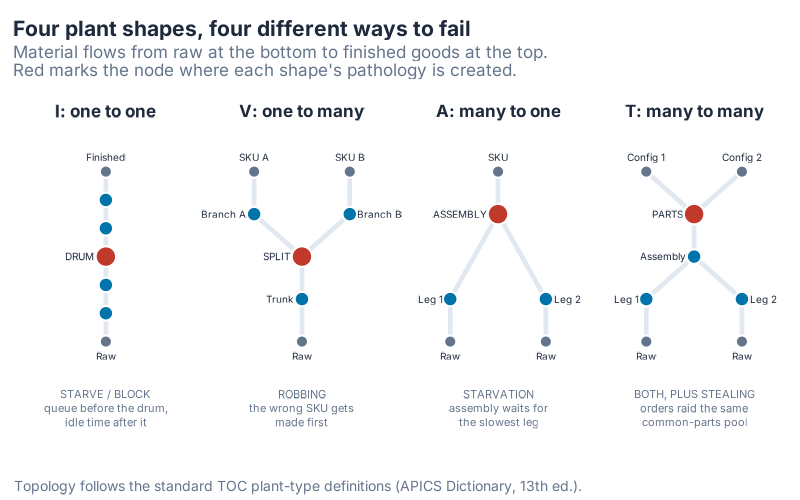
The red dot marks where each shape’s characteristic failure gets created. In the I-plant that node is the bottleneck itself. In the other three it isn’t. That gap is the whole point.
To show that rather than assert it, everything below comes from one deterministic simulation written for this post. One tick loop, four graphs. Nothing about the pathologies is scripted: they emerge from three rules. Convergence nodes fire on min() across all input legs. Divergence nodes let the priority branch claim first. Shared buffers get drawn down first-come-first-served. These are simulation outputs from a teaching model, not industry data, and the R code that produces every number is at the bottom of the post.
I-plant: the honest shape
Three words from Goldratt’s vocabulary carry the rest of this post. The drum is the slowest resource. Everything else marches to its beat. The rope is the discipline of releasing material at the drum’s rate and no faster, so the front of the line can’t outrun the middle. A buffer is stock you park in front of something you refuse to let starve.
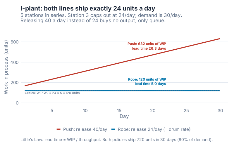
Five stations in series. Capacities of 40, 40, 24, 40, 40 units a day. Station 3 is the drum at 24 a day. Demand is 30 a day, so the plant is short on capacity before we start.
One lever, and only one. How fast do you release raw material at the front? Push means 40 a day, station 1’s capacity, because idle machines look bad. Rope means 24 a day, the drum rate. Anything above that buys queue, not output.
| Metric, day 30 | Push (release 40) | Rope (release 24) |
|---|---|---|
| Throughput | 24 units/day | 24 units/day |
| Units shipped, 30 days | 720 | 720 |
| Demand filled | 80.0% | 80.0% |
| WIP | 632 units | 120 units |
| Lead time (Little’s Law) | 26.3 days | 5.0 days |
Both policies ship 720 units. Both fill 80.0% of demand. The push policy buys you 512 extra units of inventory and a lead time of 26.3 days instead of 5.0, and not one extra unit out the door. Of the 632 units of push WIP, 504 sit in front of station 3 in a queue that does nothing except age.
What jumped out at me is where the rope lands. Not just lower. It settles at 120 units and holds there, which is the critical WIP exactly: bottleneck rate times raw process time, 24 times 5. The line finds its own floor. You don’t have to tune that number, you have to stop overriding it.
This is the shape everyone already understands, and it’s here as a baseline. The customer still gets 80.0% of what they ordered, and no release policy on earth fixes that, because the loss is genuine missing capacity. Remember that sentence. It stops being true two shapes from now.
A-plant: the leg at 100% utilisation is the problem
Two legs feed one assembly. Leg 1 makes 50 a day, leg 2 makes 30 a day, assembly can do 100 a day and is nowhere near the constraint. Assembly fires min(capacity, leg 1 buffer, leg 2 buffer) and consumes from both legs, because you can’t ship half a product.
So assembly runs at 30 a day. Leg 2’s rate. That part is intuitive.
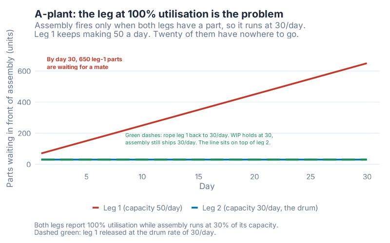
Here’s the part that isn’t. Leg 1 keeps making 50 a day, assembly consumes 30 a day, and the difference has to go somewhere. It goes into a pile that grows by 20 units every single day, reaching 650 units by day 30. A part entering leg 1 now waits 21.7 days in front of assembly before it finds a mate. Little’s Law again: 650 divided by 30.
Now read the utilisation report for that month:
| Resource | Utilisation, push policy |
|---|---|
| Leg 1 | 100.0% |
| Leg 2 | 100.0% |
| Assembly | 30.0% |
Two resources at 100%, and the one that touches the customer at 30%. Leg 1 made 1,500 parts. 900 got assembled. The rest became inventory, and the report calling leg 1 your best-performing cell is describing the cause.
Rope leg 1 back to the drum rate and leg-1 WIP holds at 30 units instead of 650. On the chart, that green dashed line sits exactly on top of the leg 2 line, which looks like a plotting error and is in fact the entire point: rope the fast leg to the slow leg and the two behave identically. Same 900 units shipped either way. Same 60.0% of demand filled.
So the A-plant is the I-plant’s lesson wearing a costume. The pathology moved, the arithmetic didn’t.
V-plant: the same 300 units, seen three ways
Now the shapes start lying to you.
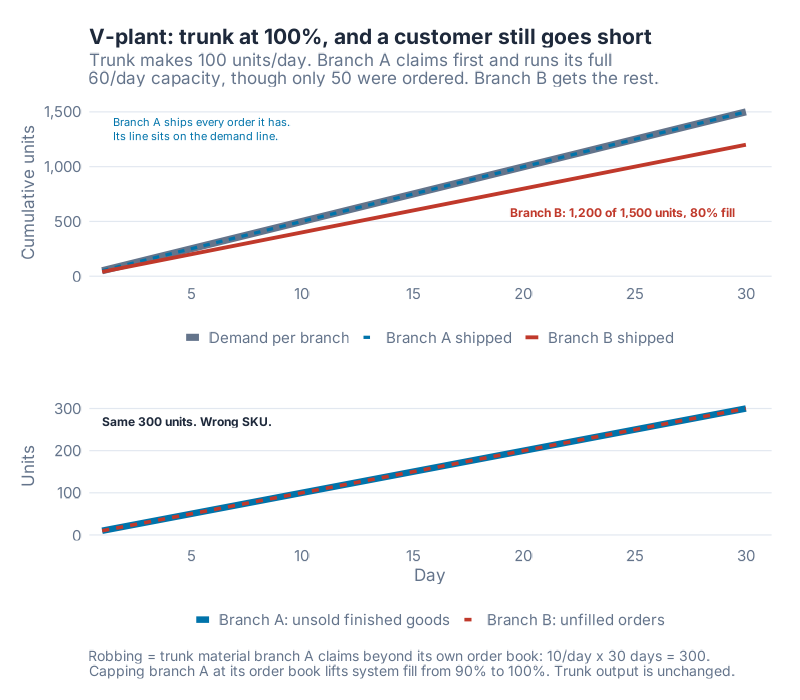
One trunk at 100 units a day splits into two branches, each able to run 60 a day, each selling 50 a day. Total demand is 100. Trunk capacity is 100. On paper this plant is balanced to the unit and has no problem at all.
Branch A draws from the divergence buffer first. That priority is the whole problem. Greedy, it claims what its cell can run, 60 a day, against an order book of 50. Branch B takes the remainder, 40 a day, against orders of 50.
Trunk utilisation: 100.0%, both policies. System throughput: 100 units a day, both policies. Not one unit of conversion is lost.
And the system fill rate is 90.0%. Branch A fills 100.0% of its orders. Branch B fills 80.0%.
Over 30 days, branch A claims 300 units beyond its own order book. TOC has a word for this. It isn’t a gentle one: robbing. The mechanism is worth restating, because it’s what separates this shape from the two above. The operation just after the fork takes material meant for its sibling. And once that material has gone down the wrong branch, it doesn’t come back without significant rework.
That last point is the whole difference. In an I-plant or an A-plant, excess work in process is early. In a V-plant, excess work in process is wrong, and steel that became one product does not become a different product on Monday.
Look at the bottom panel of that chart again. Branch A’s unsold finished goods and branch B’s unfilled orders are two lines that lie on top of each other for thirty straight days, both landing on 300. They aren’t two problems. They’re one transaction:
- 300 units robbed from the trunk
- = 300 units of branch B backlog
- = 300 units of branch A dead stock
The same 300 units, counted from three sides. Cap branch A at its order book and robbing goes to zero, both branches fill 100.0%, system fill goes from 90.0% to 100.0%, and the trunk keeps converting the identical 100 units a day it always did.
Nobody bought a machine. Nobody worked a weekend.
T-plant: 450 stolen parts, 390 missed orders, and a clean inventory report
The T is where both failure modes live in one plant, which is why practitioner literature generally treats it as the trickiest of the four to schedule.
Two legs run 65 a day each into a common-parts assembly capped at 60 a day, the drum. Common parts land on a shared shelf primed with 120 units, two days of cover. Two configuration cells draw from that same shelf, 45 a day of capacity each, and each configuration sells 30 a day. Order book: 60 a day. Common-parts supply: 60 a day. Balanced again, on paper, again.
Config 1 draws first. Greedy, it draws 45 against orders of 30.
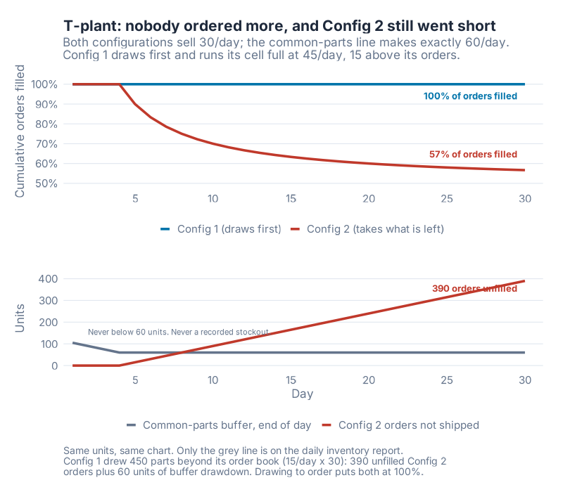
Config 1 fills 100.0% of its orders and ships complete on 30 of 30 days. Config 2 fills 56.7% and ships complete on 4 of 30 days. System fill: 78.3%.
Now the reconciliation, and don’t let anyone hand-wave this one. Config 1 drew 450 parts beyond its own order book. Config 2 finished the month 390 orders short. Those are not the same number. The gap is the interesting part:
450 stolen = 390 unfilled Config 2 orders + 60 units of buffer drawn down.
The shelf absorbed the first 60 units of theft. It fell from 120 to 60 across the opening four days, which is exactly why Config 2 shipped complete on those four days and never again. A buffer doesn’t prevent theft. It delays the invoice.
And here is the sentence I’d put on the wall of any planning office. The common-parts buffer ended the day at a minimum of 60 units, a mean of 63.0, and a maximum of 105. It ended a day empty on 0 of 30 days. There is no stockout in this data. Not one. Every inventory KPI you’d normally trust reported a healthy shelf all month while Config 2’s customer received 56.7% of their order, because the theft happens within the day, at the moment of the draw, and end-of-day snapshots are blind to it.
The A-side of the T is misbehaving at the same time: the legs make 65 a day against a 60 a day assembly, so each leg’s WIP grows by 5 a day and hits 215 units by day 30. Both diseases, one plant, one month.
Config 1 draws to order instead, and Config 2 goes from 56.7% to 100.0%. That’s +43.3 percentage points, out of a plant that converted 60 units a day before and 60 units a day after.
The punchline: the fix converts nothing
Put all four next to each other.
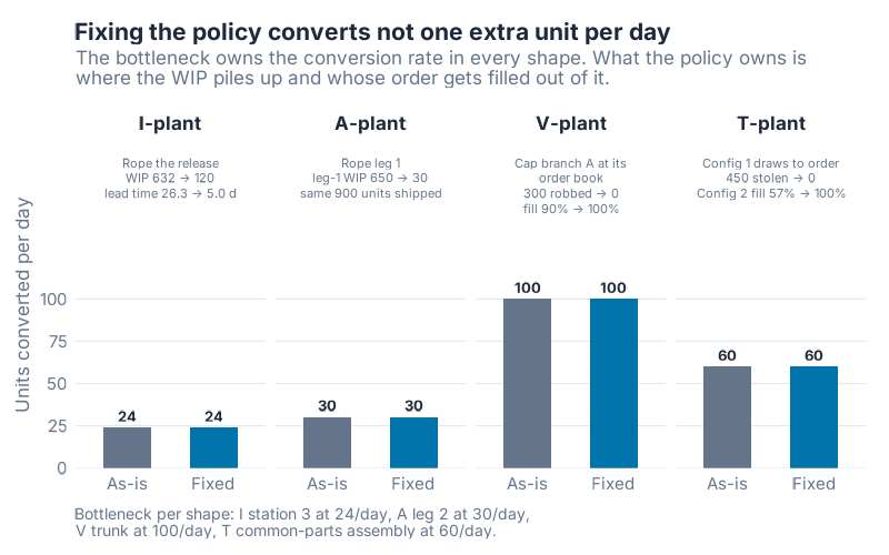
| Shape | Bottleneck | Throughput, as-is | Throughput, fixed | What the fix actually changes |
|---|---|---|---|---|
| I | station 3, 24/day | 24/day | 24/day | WIP 632 → 120; lead time 26.3 → 5.0 days |
| A | leg 2, 30/day | 30/day | 30/day | leg-1 WIP 650 → 30; same 900 units shipped |
| V | trunk, 100/day | 100/day | 100/day | 300 robbed → 0; system fill 90% → 100% |
| T | common assembly, 60/day | 60/day | 60/day | 450 stolen → 0; Config 2 fill 57% → 100% |
Fixing the policy converts not one extra unit per day in any of the four shapes. The bottleneck owns the conversion rate, always, in every topology. That law never bends.
What the policy owns is where the WIP sits and whose order gets filled.
Now hold those two halves apart, because blurring them is how this insight gets misquoted. In the I-plant and the A-plant, the fix changes WIP and lead time and nothing else. Units shipped stay at 720 and 900, fill rate stays at 80.0% and 60.0%, and the customer’s shortfall there is a real capacity shortfall that no scheduling policy recovers. In the V-plant and the T-plant, conversion also stays flat, 100 and 60 units a day, and yet delivered output moves: system fill goes 90.0% to 100.0% and 78.3% to 100.0%. Same law, opposite conclusion, because the V and T losses were never about capacity. They were misallocation.
Take one thing from this post? Take the gap between those two halves.
Which leads to a claim I’ll defend. Utilisation is not a performance metric in a V, A or T plant. It’s a warning light. The most dangerous machine on your floor isn’t the slow one, it’s the fast one standing just after a fork, and every efficiency report you own is currently congratulating it.
Where the buffers go, by shape
This is what VATI is for. Not taxonomy for its own sake: an answer to where you put the drum, the buffers and the rope. Those three together are the TOC scheduling method, drum-buffer-rope (DBR), and its buffer taxonomy is standard. A constraint buffer protects the drum from starving, a shipping buffer protects the due date, an assembly buffer protects a convergence point from a late non-constraint leg. With no internal constraint, DBR degenerates to shipping buffer alone, which is Simplified DBR.
The per-shape mapping below recurs across TOC practitioner literature rather than sitting in one quotable primary instruction. Treat it as a strong starting position, not scripture.
| Shape | Drum | Buffers that matter | The discipline that fails first |
|---|---|---|---|
| I | The slow station, and it’s obvious | Constraint buffer, shipping buffer | Releasing faster than the drum |
| V | At or before the base of the V | Constraint buffer, shipping buffer | Letting the operation right after the split batch to its own capacity |
| A | Anywhere in the converging network | Constraint, shipping, plus an assembly buffer at final assembly | Judging a feeder leg on its own utilisation |
| T | Usually the common-parts point | All three, at the common-parts store | Both of the above, at once |
The A-plant’s assembly buffer is the one people skip. A perfectly scheduled drum still starves final assembly if a non-constraint leg is late, and in our A-plant scenario the leg with the runaway pile was the one nobody was worried about.
Where this breaks
I’m not going to hand you a dollar figure from this model, and you should be suspicious of anyone who does with theirs. Here’s what it can’t do.
Real plants are not pure letters. Every source stresses this. Actual factories are hybrids: a V-base with a T-top, an A-base feeding a V, a T that behaves like an I until the last week of the month. The letter describes the dominant flow of one product family. Not the site. Run the exercise per family and expect different answers.
The model has no variability. No breakdowns, no scrap, no setup times, no rework, no supplier misses, no demand noise. That’s deliberate. It proves the pathologies are structural rather than bad luck: strip out every random element and robbing and stealing still show up. Add variability and they get worse. But don’t read 26.3 days or 21.7 days as a forecast of anything.
Demand is flat and the plants are balanced on paper. The V and T scenarios were built so supply exactly equals total demand. That is the cleanest possible case, and the one most likely to make a planner call the plant healthy. Real order books are lumpy. Priorities are real too, and sometimes branch A should be served first. The point isn’t that priority is wrong. It’s that priority applied to capacity instead of to orders is what turns into theft.
The fix here is one line of policy, and in a real plant it’s a fight. Telling a cell to run below its capacity because the order book says so contradicts every local efficiency measure that cell is judged on. That conversation is harder than the maths.
Interactive Dashboard
Reading about robbing is one thing. Watching a branch eat a month of someone else’s orders while the trunk utilisation readout holds at 100.0% and refuses to move is more convincing. Four tabs, one engine. Drag any station’s capacity, switch the policy, and scrub through all thirty days. Start on the V tab: change no capacity at all, switch to Pull, and watch branch B climb back to 100% on the same machines.
Interactive Dashboard
Explore the data yourself. Adjust the parameters and watch the results update in real time.
Your next steps
Five things, and the first four fit in one afternoon.
-
Print the routings for your top 20 SKUs by volume. Pull them straight out of the ERP routing and BOM tables. Lay them out with raw material at the bottom, finished goods at the top, one dot per operation. Don’t clean them up. The messy version is the true one.
-
Mark every fork and every merge. A fork is any operation whose output feeds two different next operations. A merge is any operation that can’t start until two feeders both deliver. Count them and write the two totals down. More forks than merges means a V. More merges than forks means an A. Roughly equal numbers of both, with the merges low in the routing and the forks stacked above them after a common-parts pool, means a T. Close to zero of both means an I.
-
At each fork, ask one question: what does the next operation run against? Its own capacity and standard batch size, or a specific customer order? If the answer is capacity, you have robbing, and the units are already sitting somewhere in finished goods with the wrong label on them.
-
Put finished-goods on-hand next to backlog, by SKU, by day, for the last 90 days. Robbing has a signature and it’s a mirror image: dead stock climbing on one SKU while its sibling from the same fork accumulates backlog, on the same days, at close to the same rate. Sort by that pairing. In our simulation, both lines hit 300.
-
Check whether your buffer report could even see this. If you monitor shared inventory as an end-of-day average, run the T-plant numbers past it: minimum 60, mean 63.0, empty on 0 of 30 days, and a customer at 56.7% fill. Add a per-order-line fill rate at the point of the draw, split by which order got there first. That single column is what turns an invisible problem into an argument you can win.
Then open the simulator, set it to your shape, and move the bottleneck around until the chart looks like your last quarter. That’s usually the moment the letter stops being an acronym.
Show R Code
# =============================================================================
# generate_vati_images.R
# VATI analysis (Theory of Constraints plant shapes V, A, T, I)
# Reference deterministic tick simulation + all static images for the post.
#
# CONTRACT NOTE (v1.0, frozen 2026-08-16):
#   This script is the single source of truth for every number in the blog post
#   and in Charlie's JS dashboard. The engine is fully deterministic (no RNG),
#   integer-valued, and specified so a JS port reproduces it exactly.
#
#   UNIVERSAL TICK ORDER (1 tick = 1 day), identical for all four shapes:
#     1. Demand arrives:  need_i = backlog_i + demand_i(t)
#     2. Process every production node in REVERSE topological order
#        (most-downstream node first, most-upstream last).
#          - linear node      : fire = min(cap, input_buffer)
#          - convergence node : fire = min(cap, input_buffer_1, ..., input_buffer_K)
#                               and consume `fire` from EVERY input leg
#          - divergence node  : allocate the shared parent buffer to the child
#                               branches by the allocation policy, in priority order
#     3. Ship: shipped_i = min(FG_i, need_i); FG_i -= shipped_i
#              backlog_i = need_i - shipped_i          (shipping is uncapacitated)
#     4. Release raw material into the most-upstream buffer(s) at the release rate
#        (raw material is never short)
#     5. Record metrics
#
#   Because each node moves material exactly one step per tick, a routing of D
#   nodes has a raw process time of D days. All intermediate buffers are PRIMED
#   at t = 0 to their steady-state values ("the plant was already running
#   yesterday") so day 1 is already in steady state and every 30-day total is a
#   clean multiple of the daily rate.
#
# Run from project root:  Rscript Scripts/generate_vati_images.R
# =============================================================================

source("Scripts/theme_inphronesys.R")

suppressPackageStartupMessages({
  library(ggplot2)
  library(dplyr)
  library(tidyr)
  library(scales)
  library(patchwork)
})

# Match showtext's rendering dpi to the ggsave dpi, otherwise every string is
# drawn ~4% larger than the layout engine reserved space for and long titles,
# captions and facet strips run off the right edge of an 800px canvas.
showtext::showtext_opts(dpi = 100)

DAYS <- 30
OUT  <- "Images"
if (!dir.exists(OUT)) dir.create(OUT)

# Deterministic. No RNG is used anywhere in this script; set.seed() is called
# only to make that explicit and to guarantee reproducibility if the model is
# ever extended with variability.
set.seed(42)

fmt <- function(x, d = 0) formatC(x, format = "f", digits = d, big.mark = ",")

# =============================================================================
# 1. I-PLANT  -- linear line, 5 stations, one drum
# =============================================================================
# Stations 1..5 in series. Station 3 is the drum (cap 24 < demand 30).
# Policy lever: release rate.
#   "push" : release at station-1 capacity (40/day)  -> keep everyone busy
#   "rope" : release at the drum rate (24/day)       -> DBR
# ---------------------------------------------------------------------------
sim_i <- function(caps = c(40, 40, 24, 40, 40),
                  release = 40,
                  demand = 30,
                  days = DAYS) {
  n <- length(caps)
  # Steady-state flow reaching each station = running min of upstream caps and release
  flow <- pmin(cummin(caps), release)
  buf  <- flow            # primed: each station's tick-1 workload is waiting
  fg   <- 0
  backlog <- 0
  rec <- vector("list", days)

  for (t in seq_len(days)) {
    need <- backlog + demand                       # 1. demand arrives
    for (s in n:1) {                               # 2. reverse topological order
      moved  <- min(caps[s], buf[s])
      buf[s] <- buf[s] - moved
      if (s == n) fg <- fg + moved else buf[s + 1] <- buf[s + 1] + moved
    }
    shipped <- min(fg, need)                       # 3. ship
    fg      <- fg - shipped
    backlog <- need - shipped
    buf[1]  <- buf[1] + release                    # 4. release raw
    rec[[t]] <- data.frame(                        # 5. record
      day = t, shipped = shipped, backlog = backlog, fg = fg,
      wip = sum(buf), b1 = buf[1], b2 = buf[2], b3 = buf[3],
      b4 = buf[4], b5 = buf[5]
    )
  }
  out <- bind_rows(rec)
  out$cum_shipped <- cumsum(out$shipped)
  out$cum_demand  <- cumsum(rep(demand, days))
  # Little's Law: lead time = WIP / throughput
  out$lead_time <- out$wip / out$shipped
  out
}

i_push <- sim_i(release = 40)
i_rope <- sim_i(release = 24)

# =============================================================================
# 2. A-PLANT  -- two converging legs feeding one assembly
# =============================================================================
# Leg 1 cap 50 (healthy), Leg 2 cap 30 (the drum), assembly cap 100.
# Assembly fires min(cap, leg1_buffer, leg2_buffer) -> the convergence rule.
# Policy lever: leg-1 release rate.
#   "push" : leg 1 released at its own capacity (50/day) -> local efficiency
#   "rope" : leg 1 released at the drum rate (30/day)    -> DBR
# ---------------------------------------------------------------------------
sim_a <- function(cap_leg = c(50, 30),
                  cap_asm = 100,
                  release = c(50, 30),
                  demand = 50,
                  days = DAYS) {
  drum <- min(cap_asm, min(pmin(cap_leg, release)))
  buf  <- pmin(cap_leg, release)   # primed at each leg's tick-1 output
  fg <- 0; backlog <- 0
  rec <- vector("list", days)

  for (t in seq_len(days)) {
    need <- backlog + demand                            # 1.
    asm  <- min(cap_asm, buf[1], buf[2])                # 2. convergence: min()
    buf  <- buf - asm                                   #    consume from EVERY leg
    fg   <- fg + asm
    shipped <- min(fg, need)                            # 3.
    fg      <- fg - shipped
    backlog <- need - shipped
    buf <- buf + pmin(cap_leg, release)                 # 4. legs produce/release
    rec[[t]] <- data.frame(
      day = t, assembled = asm, shipped = shipped, backlog = backlog,
      wip_leg1 = buf[1], wip_leg2 = buf[2], wip = sum(buf) + fg
    )
  }
  out <- bind_rows(rec)
  out$cum_shipped <- cumsum(out$shipped)
  out$cum_demand  <- cumsum(rep(demand, days))
  out$drum <- drum
  out
}

a_push <- sim_a(release = c(50, 30))
a_rope <- sim_a(release = c(30, 30))

# =============================================================================
# 3. V-PLANT  -- one trunk diverging into two branches
# =============================================================================
# Trunk cap 100/day feeds a divergence buffer. Branch A (cap 60) has priority
# and claims FIRST; branch B gets the remainder. Demand 50/day per branch, so
# total demand (100) exactly equals trunk capacity: on paper the plant is
# perfectly balanced.
# Policy lever: what branch A is allowed to claim.
#   "greedy" : claim min(cap_A, buffer)             -> runs to capacity (60), robs B
#   "pull"   : claim min(cap_A, need_A, buffer)     -> claims only what is ordered
# ---------------------------------------------------------------------------
sim_v <- function(cap_trunk = 100,
                  cap_branch = c(60, 60),
                  demand = c(50, 50),
                  policy = c("greedy", "pull"),
                  days = DAYS) {
  policy <- match.arg(policy)
  divbuf <- cap_trunk           # primed with one tick of trunk output
  fg <- c(0, 0); backlog <- c(0, 0)
  rec <- vector("list", days)

  for (t in seq_len(days)) {
    need <- backlog + demand                            # 1.
    claim <- c(0, 0)                                    # 2. divergence allocation
    for (b in 1:2) {                                    #    priority order: A then B
      want <- if (policy == "greedy") cap_branch[b] else min(cap_branch[b], need[b])
      claim[b] <- min(want, divbuf)
      divbuf   <- divbuf - claim[b]
      fg[b]    <- fg[b] + claim[b]
    }
    shipped <- pmin(fg, need)                           # 3.
    fg      <- fg - shipped
    backlog <- need - shipped
    trunk_out <- cap_trunk                              # 4. trunk (raw never short)
    divbuf    <- divbuf + trunk_out
    rec[[t]] <- data.frame(
      day = t, trunk_out = trunk_out,
      claim_A = claim[1], claim_B = claim[2],
      ship_A = shipped[1], ship_B = shipped[2],
      fg_A = fg[1], fg_B = fg[2],
      backlog_A = backlog[1], backlog_B = backlog[2],
      divbuf = divbuf
    )
  }
  out <- bind_rows(rec)
  out$cum_ship_A   <- cumsum(out$ship_A)
  out$cum_ship_B   <- cumsum(out$ship_B)
  out$cum_demand   <- cumsum(rep(demand[1], days))
  # "Robbed" units: trunk material claimed by branch A beyond branch A's own
  # same-day requirement. Under the pull policy this is 0 by construction.
  out$robbed       <- pmax(0, out$claim_A - demand[1])
  out$cum_robbed   <- cumsum(out$robbed)
  out$trunk_util   <- out$trunk_out / cap_trunk
  out
}

v_greedy <- sim_v(policy = "greedy")
v_pull   <- sim_v(policy = "pull")

# =============================================================================
# 4. T-PLANT  -- two legs converge to common parts, then diverge into configs
# =============================================================================
# Legs cap 65 each -> common-parts assembly cap 60 (the drum) -> shared
# common-parts buffer (primed at 120 = 2 days of cover) -> two configuration
# branches (cap 45 each) drawing from the SAME buffer, Config 1 first (FCFS).
# Both configurations sell 30/day, so the order book (60/day) exactly matches
# the common-parts supply (60/day). The plant can serve everybody.
# Policy lever: what Config 1 is allowed to draw.
#   "greedy" : draw min(cap_1, buffer)          -> configure cell runs full (45/day)
#   "pull"   : draw min(cap_1, need_1, buffer)  -> draw only against real orders
# Config 2 always pulls; it takes whatever is left on the shelf.
# ---------------------------------------------------------------------------
t_demand_c1 <- rep(30, DAYS)
t_demand_c2 <- rep(30, DAYS)

sim_t <- function(cap_leg = c(65, 65),
                  cap_common = 60,
                  cap_cfg = c(45, 45),
                  buffer0 = 120,
                  d1 = t_demand_c1,
                  d2 = t_demand_c2,
                  policy = c("greedy", "pull"),
                  days = DAYS) {
  policy <- match.arg(policy)
  legbuf <- cap_leg                    # primed at each leg's tick-1 output
  cpbuf  <- buffer0                    # shared common-parts buffer
  fg <- c(0, 0); backlog <- c(0, 0)
  rec <- vector("list", days)

  for (t in seq_len(days)) {
    need <- backlog + c(d1[t], d2[t])                   # 1.
    # 2a. divergence off the SHARED buffer, priority order: Config 1 then Config 2
    want1 <- if (policy == "greedy") cap_cfg[1] else min(cap_cfg[1], need[1])
    draw  <- c(0, 0)
    draw[1] <- min(want1, cpbuf)
    after_c1 <- cpbuf - draw[1]        # what is left on the shelf for Config 2
    draw[2] <- min(cap_cfg[2], need[2], after_c1)
    cpbuf   <- after_c1 - draw[2]
    trough  <- cpbuf                   # within-day low point
    fg      <- fg + draw

    common <- min(cap_common, legbuf[1], legbuf[2])     # 2b. convergence: min()
    legbuf <- legbuf - common
    cpbuf  <- cpbuf + common

    shipped <- pmin(fg, need)                           # 3. ship
    fg      <- fg - shipped
    backlog <- need - shipped

    legbuf <- legbuf + cap_leg                          # 4. legs release
    rec[[t]] <- data.frame(
      day = t, demand_1 = d1[t], demand_2 = d2[t],
      draw_1 = draw[1], draw_2 = draw[2],
      ship_1 = shipped[1], ship_2 = shipped[2],
      fg_1 = fg[1], fg_2 = fg[2],
      backlog_1 = backlog[1], backlog_2 = backlog[2],
      common_out = common, cp_end = cpbuf,
      cp_after_c1 = after_c1, cp_trough = trough,
      wip_leg1 = legbuf[1], wip_leg2 = legbuf[2]
    )
  }
  out <- bind_rows(rec)
  out$cum_ship_1 <- cumsum(out$ship_1); out$cum_dem_1 <- cumsum(out$demand_1)
  out$cum_ship_2 <- cumsum(out$ship_2); out$cum_dem_2 <- cumsum(out$demand_2)
  out$fill_1 <- out$cum_ship_1 / out$cum_dem_1
  out$fill_2 <- out$cum_ship_2 / out$cum_dem_2
  # "Stolen" units: common parts drawn by Config 1 beyond Config 1's own orders.
  # Supply (60/day) exactly equals combined demand (30 + 30), so every stolen
  # part is a part Config 2 was entitled to.
  out$stolen     <- pmax(0, out$draw_1 - out$demand_1)
  out$cum_stolen <- cumsum(out$stolen)
  out
}

t_greedy <- sim_t(policy = "greedy")
t_pull   <- sim_t(policy = "pull")

# =============================================================================
# NUMERIC SUMMARY -- every number allowed to appear in the post
# =============================================================================
line <- function(...) cat(..., "\n", sep = "")
rule <- function(ch = "=") cat(strrep(ch, 78), "\n", sep = "")

rule(); line("VATI REFERENCE SIMULATION  |  v1.0  |  ", DAYS, " ticks (days), deterministic"); rule()

# ---- I ----
line("\n[I-PLANT] 5 stations in series, caps 40/40/24/40/40, demand 30/day")
i_last_push <- tail(i_push, 1); i_last_rope <- tail(i_rope, 1)
line("  drum (station 3) capacity ............ 24 units/day")
line("  PUSH release 40/day:")
line("    throughput (steady state) .......... ", i_last_push$shipped, " units/day")
line("    30-day units shipped ............... ", fmt(i_last_push$cum_shipped))
line("    demand filled ...................... ", fmt(100 * i_last_push$cum_shipped / i_last_push$cum_demand, 1),
     "%   (", fmt(i_last_push$cum_shipped), " / ", fmt(i_last_push$cum_demand), ")")
line("    WIP at day 30 ...................... ", fmt(i_last_push$wip), " units")
line("      of which queued at the drum ...... ", fmt(i_last_push$b3), " units")
line("    lead time (Little's Law WIP/TH) .... ", fmt(i_last_push$lead_time, 1), " days   (",
     fmt(i_last_push$wip), " / ", i_last_push$shipped, ")")
line("  ROPE release 24/day (= drum rate):")
line("    throughput (steady state) .......... ", i_last_rope$shipped, " units/day")
line("    30-day units shipped ............... ", fmt(i_last_rope$cum_shipped))
line("    demand filled ...................... ", fmt(100 * i_last_rope$cum_shipped / i_last_rope$cum_demand, 1), "%")
line("    WIP at day 30 ...................... ", fmt(i_last_rope$wip), " units")
line("    lead time (Little's Law WIP/TH) .... ", fmt(i_last_rope$lead_time, 1), " days   (",
     fmt(i_last_rope$wip), " / ", i_last_rope$shipped, ")")
line("  Critical WIP W0 = bottleneck rate x raw process time = 24 x 5 = ", 24 * 5, " units")
line("  WIP removed by the rope ............... ", fmt(i_last_push$wip - i_last_rope$wip), " units (",
     fmt(100 * (1 - i_last_rope$wip / i_last_push$wip), 1), "% less)")
line("  Lead time cut ......................... ", fmt(i_last_push$lead_time, 1), " -> ",
     fmt(i_last_rope$lead_time, 1), " days")

# ---- A ----
line("\n[A-PLANT] 2 legs (cap 50 / 30) -> assembly (cap 100), demand 50/day")
a_lp <- tail(a_push, 1); a_lr <- tail(a_rope, 1)
line("  assembly throughput = slowest leg ..... ", a_lp$assembled, " units/day  (leg 2 cap = 30)")
line("  PUSH (leg 1 released at its own capacity 50/day):")
line("    30-day units shipped ............... ", fmt(a_lp$cum_shipped))
line("    demand filled ...................... ", fmt(100 * a_lp$cum_shipped / a_lp$cum_demand, 1),
     "%   (", fmt(a_lp$cum_shipped), " / ", fmt(a_lp$cum_demand), ")")
line("    leg-1 WIP in front of assembly, d30  ", fmt(a_lp$wip_leg1), " units")
line("    leg-2 WIP in front of assembly, d30  ", fmt(a_lp$wip_leg2), " units")
line("    leg-1 WIP growth rate .............. +", 50 - a_lp$assembled, " units/day (50 made - 30 consumed)")
line("    leg-1 utilisation .................. 100.0%  (50 / 50)")
line("    leg-2 utilisation .................. 100.0%  (30 / 30)")
line("    assembly utilisation ............... ", fmt(100 * a_lp$assembled / 100, 1), "%  (30 / 100)")
line("    dwell time of a leg-1 part (W/TH) .. ", fmt(a_lp$wip_leg1 / a_lp$assembled, 1), " days   (",
     fmt(a_lp$wip_leg1), " / ", a_lp$assembled, ")")
line("    parts leg 1 made / assembled ....... ", fmt(sum(pmin(50, 50)) * DAYS), " / ", fmt(a_lp$cum_shipped))
line("  ROPE (leg 1 released at the drum rate 30/day):")
line("    30-day units shipped ............... ", fmt(a_lr$cum_shipped), "  (unchanged)")
line("    leg-1 WIP in front of assembly, d30  ", fmt(a_lr$wip_leg1), " units")
line("    leg-1 utilisation .................. ", fmt(100 * 30 / 50, 1), "%  (30 / 50)")
line("  WIP removed by the rope ............... ", fmt(a_lp$wip_leg1 - a_lr$wip_leg1), " units")

# ---- V ----
line("\n[V-PLANT] trunk cap 100 -> branch A (cap 60) + branch B (cap 60), demand 50 + 50")
v_lg <- tail(v_greedy, 1); v_lp <- tail(v_pull, 1)
line("  trunk utilisation ..................... ", fmt(100 * mean(v_greedy$trunk_util), 1), "%")
line("  system throughput ..................... ", v_lg$claim_A + v_lg$claim_B, " units/day (both policies)")
line("  GREEDY branch A (claims to capacity):")
line("    branch A claims .................... ", v_lg$claim_A, " units/day (demand 50)")
line("    branch B receives .................. ", v_lg$claim_B, " units/day (demand 50)")
line("    30-day shipped A / B ............... ", fmt(v_lg$cum_ship_A), " / ", fmt(v_lg$cum_ship_B))
line("    branch A fill rate ................. ", fmt(100 * v_lg$cum_ship_A / v_lg$cum_demand, 1), "%")
line("    branch B fill rate ................. ", fmt(100 * v_lg$cum_ship_B / v_lg$cum_demand, 1),
     "%   (", fmt(v_lg$cum_ship_B), " / ", fmt(v_lg$cum_demand), ")")
line("    system fill rate ................... ",
     fmt(100 * (v_lg$cum_ship_A + v_lg$cum_ship_B) / (2 * v_lg$cum_demand), 1), "%   (",
     fmt(v_lg$cum_ship_A + v_lg$cum_ship_B), " / ", fmt(2 * v_lg$cum_demand), ")")
line("    units robbed (cumulative) .......... ", fmt(v_lg$cum_robbed), " units  (10/day x 30)")
line("    branch A excess finished goods ..... ", fmt(v_lg$fg_A), " units")
line("    branch B backlog at day 30 ......... ", fmt(v_lg$backlog_B), " units")
line("  PULL branch A (claims only what is ordered):")
line("    branch A claims .................... ", v_lp$claim_A, " units/day")
line("    branch B receives .................. ", v_lp$claim_B, " units/day")
line("    branch A / B fill rate ............. ", fmt(100 * v_lp$cum_ship_A / v_lp$cum_demand, 1), "% / ",
     fmt(100 * v_lp$cum_ship_B / v_lp$cum_demand, 1), "%")
line("    system fill rate ................... ",
     fmt(100 * (v_lp$cum_ship_A + v_lp$cum_ship_B) / (2 * v_lp$cum_demand), 1), "%")
line("    units robbed ....................... ", fmt(v_lp$cum_robbed))
line("    branch A excess FG / branch B backlog ", fmt(v_lp$fg_A), " / ", fmt(v_lp$backlog_B))

# ---- T ----
line("\n[T-PLANT] legs 65/65 -> common assembly cap 60 -> shared buffer (120) -> configs 45/45")
line("  Config 1 and Config 2 each sell 30/day. Order book (60) == common-parts supply (60).")
t_lf <- tail(t_greedy, 1); t_lp <- tail(t_pull, 1)
line("  common parts produced ................. ", t_lf$common_out, " units/day  x 30 = ",
     fmt(sum(t_greedy$common_out)))
line("  total demand (C1 + C2) ................ ", fmt(t_lf$cum_dem_1 + t_lf$cum_dem_2), " units  (",
     fmt(t_lf$cum_dem_1), " + ", fmt(t_lf$cum_dem_2), ")")
line("  GREEDY Config 1 (configure cell runs full at 45/day):")
line("    Config 1 draws ..................... ", t_lf$draw_1, " units/day (orders 30)")
line("    Config 2 draws (steady state) ...... ", t_lf$draw_2, " units/day (orders 30)")
line("    Config 1 fill rate ................. ", fmt(100 * t_lf$fill_1, 1), "%   (",
     fmt(t_lf$cum_ship_1), " / ", fmt(t_lf$cum_dem_1), ")")
line("    Config 2 fill rate ................. ", fmt(100 * t_lf$fill_2, 1), "%   (",
     fmt(t_lf$cum_ship_2), " / ", fmt(t_lf$cum_dem_2), ")")
line("    system fill rate ................... ",
     fmt(100 * (t_lf$cum_ship_1 + t_lf$cum_ship_2) / (t_lf$cum_dem_1 + t_lf$cum_dem_2), 1), "%   (",
     fmt(t_lf$cum_ship_1 + t_lf$cum_ship_2), " / ", fmt(t_lf$cum_dem_1 + t_lf$cum_dem_2), ")")
line("    stolen units (C1 draw beyond orders) ", fmt(t_lf$cum_stolen), " units (15/day x 30)")
line("    Config 2 backlog at day 30 ......... ", fmt(t_lf$backlog_2), " units")
line("    RECONCILIATION: 450 stolen = ", fmt(t_lf$cum_dem_2 - t_lf$cum_ship_2),
     " unfilled orders + ", fmt(120 - t_lf$cp_end), " units of buffer drawn down")
line("    Config 1 unsold configured stock ... ", fmt(t_lf$fg_1), " units")
line("    days Config 2 shipped complete ..... ", sum(t_greedy$backlog_2 == 0), " / ", DAYS)
line("    days Config 1 shipped complete ..... ", sum(t_greedy$backlog_1 == 0), " / ", DAYS)
line("    buffer end-of-day: max ", fmt(max(t_greedy$cp_end)), " min ", fmt(min(t_greedy$cp_end)),
     " mean ", fmt(mean(t_greedy$cp_end), 1))
line("    days the buffer ended empty ........ ", sum(t_greedy$cp_end == 0), " / ", DAYS)
line("    shelf level Config 2 arrives to ..... day 1: ", t_greedy$cp_after_c1[1],
     "  -> steady state: ", t_lf$cp_after_c1)
line("    A-side leg WIP at day 30 (each) .... ", fmt(t_lf$wip_leg1), " units (+5/day, 65 made - 60 used)")
line("  PULL Config 1 (draw only against real orders):")
line("    Config 1 draws ..................... ", t_lp$draw_1, " units/day")
line("    Config 2 draws ..................... ", t_lp$draw_2, " units/day")
line("    Config 1 / Config 2 fill rate ...... ", fmt(100 * t_lp$fill_1, 1), "% / ",
     fmt(100 * t_lp$fill_2, 1), "%")
line("    system fill rate ................... ",
     fmt(100 * (t_lp$cum_ship_1 + t_lp$cum_ship_2) / (t_lp$cum_dem_1 + t_lp$cum_dem_2), 1), "%")
line("    stolen units ....................... ", fmt(t_lp$cum_stolen), " units")
line("    buffer end-of-day (flat) ........... ", t_lp$cp_end, " units")
line("    Config 2 fill improvement .......... +",
     fmt(100 * (t_lp$fill_2 - t_lf$fill_2), 1), " pp")

# ---- invariants ----
line("\n[INVARIANT CHECKS]")
line("  I: throughput == drum rate (24) ....... ",
     all(i_push$shipped == 24) && all(i_rope$shipped == 24))
line("  I: Little's Law WIP = TH x LT ......... ",
     isTRUE(all.equal(i_last_push$wip, i_last_push$shipped * i_last_push$lead_time)))
line("  I: rope WIP == critical WIP W0 = 120 .. ", i_last_rope$wip == 120)
line("  A: assembly rate == slowest leg (30) .. ",
     all(a_push$assembled == 30) && all(a_rope$assembled == 30))
line("  A: throughput identical push vs rope .. ", a_lp$cum_shipped == a_lr$cum_shipped)
line("  A: leg-1 material balance ............. ",
     50 + 50 * DAYS - 30 * DAYS == a_lp$wip_leg1)
line("  V: system throughput identical ........ ",
     (v_lg$cum_ship_A + v_lg$cum_ship_B + v_lg$fg_A) == (v_lp$cum_ship_A + v_lp$cum_ship_B + v_lp$fg_A))
line("  V: robbed == branch-B shortfall ....... ",
     v_lg$cum_robbed == (v_lg$cum_demand - v_lg$cum_ship_B))
line("  V: trunk utilisation 100% both ........ ", all(v_greedy$trunk_util == 1))
line("  T: common parts rate == 60/day ........ ",
     all(t_greedy$common_out == 60) && all(t_pull$common_out == 60))
line("  T: common-parts balance (120 + 30x60 - drawn - buffer == 0) ",
     120 + 30 * 60 - sum(t_greedy$draw_1 + t_greedy$draw_2) - t_lf$cp_end == 0)
line("  T: stolen == C2 shortfall + buffer drawdown (450 == 390 + 60) ",
     t_lf$cum_stolen == (t_lf$cum_dem_2 - t_lf$cum_ship_2) + (120 - t_lf$cp_end))
line("  T: buffer never ends a day empty ...... ", all(t_greedy$cp_end > 0))
rule()

# =============================================================================
# IMAGE 1 -- the four flow topologies
# =============================================================================
shapes <- c("I: one to one", "V: one to many",
            "A: many to one", "T: many to many")

nodes <- bind_rows(
  # All five stations are drawn, matching the five-station line in sim_i().
  data.frame(shape = shapes[1], x = 0, y = seq(0, 4, length.out = 7),
             lab = c("Raw", "", "", "DRUM", "", "", "Finished"),
             kind = c("end", "std", "std", "crit", "std", "std", "end"),
             side = c("b", "l", "l", "l", "l", "l", "t")),
  data.frame(shape = shapes[2],
             x   = c(0, 0, 0, -1, 1, -1, 1),
             y   = c(0, 1, 2,  3, 3,  4, 4),
             lab = c("Raw", "Trunk", "SPLIT", "Branch A", "Branch B", "SKU A", "SKU B"),
             kind = c("end", "std", "crit", "std", "std", "end", "end"),
             side = c("b", "l", "l", "l", "r", "t", "t")),
  data.frame(shape = shapes[3],
             x   = c(-1, 1, -1, 1, 0, 0),
             y   = c( 0, 0,  1, 1, 3, 4),
             lab = c("Raw", "Raw", "Leg 1", "Leg 2", "ASSEMBLY", "SKU"),
             kind = c("end", "end", "std", "std", "crit", "end"),
             side = c("b", "b", "l", "r", "l", "t")),
  data.frame(shape = shapes[4],
             x   = c(-1, 1, -1, 1, 0, 0, -1, 1),
             y   = c( 0, 0,  1, 1, 2, 3,  4, 4),
             lab = c("Raw", "Raw", "Leg 1", "Leg 2", "Assembly", "PARTS", "Config 1", "Config 2"),
             kind = c("end", "end", "std", "std", "std", "crit", "end", "end"),
             side = c("b", "b", "l", "r", "l", "l", "t", "t"))
)
# Labels sit outside the node, never inside it: an 800px canvas split four ways
# leaves ~200px per panel, far too little to fit a word inside a plotted point.
nodes <- nodes %>%
  mutate(
    off = ifelse(kind == "crit", 0.24, 0.16),
    lx = x + ifelse(side == "l", -off, ifelse(side == "r", off, 0)),
    ly = y + ifelse(side == "b", -0.34, ifelse(side == "t", 0.34, 0)),
    lh = ifelse(side == "l", 1, ifelse(side == "r", 0, 0.5))
  )

edge <- function(shape, x1, y1, x2, y2) data.frame(shape = shape, x = x1, y = y1, xend = x2, yend = y2)
edges <- bind_rows(
  edge(shapes[1], 0, 0, 0, 4),
  edge(shapes[2], 0, 0, 0, 1), edge(shapes[2], 0, 1, 0, 2),
  edge(shapes[2], 0, 2, -1, 3), edge(shapes[2], 0, 2, 1, 3),
  edge(shapes[2], -1, 3, -1, 4), edge(shapes[2], 1, 3, 1, 4),
  edge(shapes[3], -1, 0, -1, 1), edge(shapes[3], 1, 0, 1, 1),
  edge(shapes[3], -1, 1, 0, 3), edge(shapes[3], 1, 1, 0, 3),
  edge(shapes[3], 0, 3, 0, 4),
  edge(shapes[4], -1, 0, -1, 1), edge(shapes[4], 1, 0, 1, 1),
  edge(shapes[4], -1, 1, 0, 2), edge(shapes[4], 1, 1, 0, 2),
  edge(shapes[4], 0, 2, 0, 3),
  edge(shapes[4], 0, 3, -1, 4), edge(shapes[4], 0, 3, 1, 4)
)

captions <- data.frame(
  shape = shapes,
  x = 0, y = -1.15,
  lab = c("STARVE / BLOCK\nqueue before the drum,\nidle time after it",
          "ROBBING\nthe wrong SKU gets\nmade first",
          "STARVATION\nassembly waits for\nthe slowest leg",
          "BOTH, PLUS STEALING\norders raid the same\ncommon-parts pool")
)

nodes$shape    <- factor(nodes$shape, levels = shapes)
edges$shape    <- factor(edges$shape, levels = shapes)
captions$shape <- factor(captions$shape, levels = shapes)

p_shapes <- ggplot() +
  geom_segment(data = edges, aes(x = x, y = y, xend = xend, yend = yend),
               colour = iph_colors$lightgrey, linewidth = 1.6, lineend = "round") +
  geom_point(data = nodes, aes(x = x, y = y, fill = kind, size = kind),
             shape = 21, colour = "white", stroke = 1.1) +
  geom_text(data = nodes, aes(x = lx, y = ly, label = lab, hjust = lh),
            family = "Inter", size = 2.5, colour = iph_colors$dark) +
  geom_text(data = captions, aes(x = x, y = y, label = lab),
            family = "Inter", size = 2.8, colour = iph_colors$grey,
            lineheight = 1.05, vjust = 1) +
  scale_fill_manual(values = c(std = iph_colors$blue, crit = iph_colors$red,
                               end = iph_colors$grey), guide = "none") +
  scale_size_manual(values = c(std = 4.2, crit = 6.2, end = 3.4), guide = "none") +
  facet_wrap(~shape, nrow = 1) +
  coord_cartesian(xlim = c(-1.75, 1.75), ylim = c(-2.6, 4.7), clip = "off") +
  labs(
    title = "Four plant shapes, four different ways to fail",
    subtitle = "Material flows from raw at the bottom to finished goods at the top.\nRed marks the node where each shape's pathology is created.",
    caption = "Topology follows the standard TOC plant-type definitions (APICS Dictionary, 13th ed.)."
  ) +
  theme_inphronesys(grid = "none") +
  theme(
    axis.text = element_blank(), axis.title = element_blank(),
    panel.spacing = unit(0.6, "lines"),
    plot.margin = margin(15, 10, 4, 10)
  )

ggsave(file.path(OUT, "vati_four_shapes.png"), p_shapes,
       width = 8, height = 5, dpi = 100, bg = "white")

# =============================================================================
# IMAGE 2 -- I-plant: push vs rope
# =============================================================================
i_wip <- bind_rows(
  transform(i_push[, c("day", "wip", "shipped")], policy = "Push: release 40/day"),
  transform(i_rope[, c("day", "wip", "shipped")], policy = "Rope: release 24/day (= drum rate)")
)

p_i <- ggplot(i_wip, aes(day, wip, colour = policy)) +
  geom_line(linewidth = 1.2) +
  annotate("text", x = 22, y = i_push$wip[22] + 55,
           label = paste0("Push: ", fmt(i_last_push$wip), " units of WIP\nlead time ",
                          fmt(i_last_push$lead_time, 1), " days"),
           family = "Inter", size = 3.1, colour = iph_colors$red,
           hjust = 1, fontface = "bold", lineheight = 1.05) +
  annotate("text", x = 22, y = 210,
           label = paste0("Rope: ", fmt(i_last_rope$wip), " units of WIP\nlead time ",
                          fmt(i_last_rope$lead_time, 1), " days"),
           family = "Inter", size = 3.1, colour = iph_colors$blue,
           hjust = 1, fontface = "bold", lineheight = 1.05) +
  annotate("segment", x = 1, xend = 30, y = 120, yend = 120,
           colour = iph_colors$grey, linetype = "dotted") +
  annotate("text", x = 1, y = 100, hjust = 0,
           label = "Critical WIP W₀ = 24 × 5 = 120 units",
           family = "Inter", size = 2.8, colour = iph_colors$grey) +
  scale_colour_manual(values = c(iph_colors$red, iph_colors$blue)) +
  scale_x_continuous(breaks = seq(0, 30, 5), expand = expansion(mult = c(0.02, 0.04))) +
  scale_y_continuous(labels = comma_format(), limits = c(0, 700)) +
  labs(
    title = "I-plant: both lines ship exactly 24 units a day",
    subtitle = "5 stations in series. Station 3 caps out at 24/day; demand is 30/day.\nReleasing 40 a day instead of 24 buys no output, only queue.",
    x = "Day", y = "Work in process (units)", colour = NULL,
    caption = "Little's Law: lead time = WIP / throughput. Both policies ship 720 units in 30 days (80% of demand)."
  ) +
  theme_inphronesys(grid = "y")

ggsave(file.path(OUT, "vati_i_plant_wip_leadtime.png"), p_i,
       width = 8, height = 5, dpi = 100, bg = "white")

# =============================================================================
# IMAGE 3 -- A-plant: WIP runaway in front of assembly
# =============================================================================
a_long <- a_push %>%
  select(day, `Leg 1 (capacity 50/day)` = wip_leg1, `Leg 2 (capacity 30/day, the drum)` = wip_leg2) %>%
  pivot_longer(-day, names_to = "leg", values_to = "wip")

p_a <- ggplot(a_long, aes(day, wip, colour = leg)) +
  geom_line(linewidth = 1.2) +
  geom_line(data = data.frame(day = a_rope$day, wip = a_rope$wip_leg1),
            aes(day, wip), inherit.aes = FALSE,
            colour = iph_colors$green, linewidth = 1.3, linetype = "longdash") +
  annotate("text", x = 1.5, y = 690, hjust = 0, vjust = 1,
           label = paste0("By day 30, ", fmt(a_lp$wip_leg1), " leg-1 parts\nare waiting for a mate"),
           family = "Inter", size = 3.1, colour = iph_colors$red,
           fontface = "bold", lineheight = 1.05) +
  annotate("text", x = 8.5, y = 165, hjust = 0,
           label = paste0("Green dashes: rope leg 1 back to 30/day. WIP holds at ",
                          fmt(a_lr$wip_leg1), ",\nassembly still ships 30/day. The line sits on top of leg 2."),
           family = "Inter", size = 2.9, colour = iph_colors$green, lineheight = 1.05) +
  scale_colour_manual(values = c(iph_colors$red, iph_colors$blue)) +
  scale_x_continuous(breaks = seq(0, 30, 5), expand = expansion(mult = c(0.02, 0.04))) +
  scale_y_continuous(labels = comma_format(), limits = c(0, 720)) +
  labs(
    title = "A-plant: the leg at 100% utilisation is the problem",
    subtitle = "Assembly fires only when both legs have a part, so it runs at 30/day.\nLeg 1 keeps making 50 a day. Twenty of them have nowhere to go.",
    x = "Day", y = "Parts waiting in front of assembly (units)", colour = NULL,
    caption = "Both legs report 100% utilisation while assembly runs at 30% of its capacity.\nDashed green: leg 1 released at the drum rate of 30/day."
  ) +
  theme_inphronesys(grid = "y")

ggsave(file.path(OUT, "vati_a_plant_wip_runaway.png"), p_a,
       width = 8, height = 5, dpi = 100, bg = "white")

# =============================================================================
# IMAGE 4 -- V-plant: robbing
# =============================================================================
v_top <- v_greedy %>%
  select(day, `Branch A shipped` = cum_ship_A, `Branch B shipped` = cum_ship_B,
         `Demand per branch` = cum_demand) %>%
  pivot_longer(-day, names_to = "series", values_to = "units")
v_top$series <- factor(v_top$series,
                       levels = c("Demand per branch", "Branch A shipped", "Branch B shipped"))

p_v1 <- ggplot(v_top, aes(day, units, colour = series, linetype = series,
                          linewidth = series)) +
  geom_line() +
  annotate("text", x = 29.5, y = 620,
           label = paste0("Branch B: ", fmt(v_lg$cum_ship_B), " of ", fmt(v_lg$cum_demand),
                          " units, ", fmt(100 * v_lg$cum_ship_B / v_lg$cum_demand, 0), "% fill"),
           family = "Inter", size = 3, colour = iph_colors$red,
           hjust = 1, vjust = 1, fontface = "bold") +
  annotate("text", x = 1.5, y = 1450, hjust = 0, vjust = 1,
           label = "Branch A ships every order it has.\nIts line sits on the demand line.",
           family = "Inter", size = 2.9, colour = iph_colors$blue, lineheight = 1.05) +
  # Branch A ships exactly its demand, so the two series coincide: draw demand as a
  # thick grey line underneath and branch A dashed on top so both stay readable.
  scale_colour_manual(values = c(iph_colors$grey, iph_colors$blue, iph_colors$red)) +
  scale_linetype_manual(values = c("solid", "22", "solid")) +
  scale_linewidth_manual(values = c(2.4, 1.1, 1.3)) +
  scale_x_continuous(breaks = seq(0, 30, 5), expand = expansion(mult = c(0.02, 0.04))) +
  scale_y_continuous(labels = comma_format()) +
  labs(
    title = "V-plant: trunk at 100%, and a customer still goes short",
    subtitle = "Trunk makes 100 units/day. Branch A claims first and runs its full\n60/day capacity, though only 50 were ordered. Branch B gets the rest.",
    x = NULL, y = "Cumulative units", colour = NULL, linetype = NULL, linewidth = NULL
  ) +
  theme_inphronesys(grid = "y")

v_bot <- v_greedy %>%
  select(day, `Branch A: unsold finished goods` = fg_A,
         `Branch B: unfilled orders` = backlog_B) %>%
  pivot_longer(-day, names_to = "series", values_to = "units")

p_v2 <- ggplot(v_bot, aes(day, units, colour = series, linetype = series,
                          linewidth = series)) +
  geom_line() +
  annotate("text", x = 1, y = 270, hjust = 0,
           label = paste0("Same ", fmt(v_lg$cum_robbed), " units. Wrong SKU."),
           family = "Inter", size = 3.1, colour = iph_colors$dark, fontface = "bold") +
  # Unsold branch-A stock and unfilled branch-B orders track each other exactly:
  # solid blue underneath, red dashes on top so the coincidence is the message.
  scale_colour_manual(values = c(iph_colors$blue, iph_colors$red)) +
  scale_linetype_manual(values = c("solid", "22")) +
  scale_linewidth_manual(values = c(2.2, 1.2)) +
  scale_x_continuous(breaks = seq(0, 30, 5), expand = expansion(mult = c(0.02, 0.04))) +
  scale_y_continuous(labels = comma_format(), limits = c(0, 330)) +
  labs(x = "Day", y = "Units", colour = NULL, linetype = NULL, linewidth = NULL,
       caption = "Robbing = trunk material branch A claims beyond its own order book: 10/day x 30 days = 300.\nCapping branch A at its order book lifts system fill from 90% to 100%. Trunk output is unchanged.") +
  theme_inphronesys(grid = "y")

p_v <- p_v1 / p_v2 + plot_layout(heights = c(1.15, 1))
ggsave(file.path(OUT, "vati_v_plant_robbing.png"), p_v,
       width = 8, height = 7, dpi = 100, bg = "white")

# =============================================================================
# IMAGE 5 -- T-plant: stealing from the shared buffer
# =============================================================================
t_fill <- t_greedy %>%
  select(day, `Config 1 (draws first)` = fill_1, `Config 2 (takes what is left)` = fill_2) %>%
  pivot_longer(-day, names_to = "cfg", values_to = "fill")

p_t1 <- ggplot(t_fill, aes(day, fill, colour = cfg)) +
  geom_line(linewidth = 1.2) +
  annotate("text", x = 29.5, y = t_lf$fill_2 + 0.08,
           label = paste0(fmt(100 * t_lf$fill_2, 0), "% of orders filled"),
           family = "Inter", size = 3.2, colour = iph_colors$red,
           hjust = 1, fontface = "bold") +
  annotate("text", x = 29.5, y = 0.94,
           label = "100% of orders filled",
           family = "Inter", size = 3.2, colour = iph_colors$blue,
           hjust = 1, fontface = "bold") +
  scale_colour_manual(values = c(iph_colors$blue, iph_colors$red)) +
  scale_x_continuous(breaks = seq(0, 30, 5), expand = expansion(mult = c(0.02, 0.04))) +
  scale_y_continuous(labels = percent_format(accuracy = 1), limits = c(0.5, 1.03)) +
  labs(
    title = "T-plant: nobody ordered more, and Config 2 still went short",
    subtitle = "Both configurations sell 30/day; the common-parts line makes exactly 60/day.\nConfig 1 draws first and runs its cell full at 45/day, 15 above its orders.",
    x = NULL, y = "Cumulative orders filled", colour = NULL
  ) +
  theme_inphronesys(grid = "y")

t_buf <- t_greedy %>%
  select(day, `Common-parts buffer, end of day` = cp_end,
         `Config 2 orders not shipped` = backlog_2) %>%
  pivot_longer(-day, names_to = "series", values_to = "units")
t_buf$series <- factor(t_buf$series,
                       levels = c("Common-parts buffer, end of day", "Config 2 orders not shipped"))

p_t2 <- ggplot(t_buf, aes(day, units, colour = series)) +
  geom_line(linewidth = 1.2) +
  annotate("text", x = 2, y = 155, hjust = 0,
           label = paste0("Never below ", fmt(min(t_greedy$cp_end)),
                          " units. Never a recorded stockout."),
           family = "Inter", size = 2.9, colour = iph_colors$grey) +
  annotate("text", x = 29.5, y = t_lf$backlog_2 - 20, hjust = 1, vjust = 1,
           label = paste0(fmt(t_lf$backlog_2), " orders unfilled"),
           family = "Inter", size = 3.2, colour = iph_colors$red, fontface = "bold") +
  scale_colour_manual(values = c(iph_colors$grey, iph_colors$red)) +
  scale_x_continuous(breaks = seq(0, 30, 5), expand = expansion(mult = c(0.02, 0.04))) +
  scale_y_continuous(labels = comma_format(), limits = c(0, 440)) +
  labs(x = "Day", y = "Units", colour = NULL,
       caption = paste0("Same units, same chart. Only the grey line is on the daily inventory report.\n",
                        "Config 1 drew ", fmt(t_lf$cum_stolen),
                        " parts beyond its order book (15/day x 30): ",
                        fmt(t_lf$backlog_2), " unfilled Config 2\norders plus ",
                        fmt(120 - t_lf$cp_end),
                        " units of buffer drawdown. Drawing to order puts both at 100%.")) +
  theme_inphronesys(grid = "y")

p_t <- p_t1 / p_t2 + plot_layout(heights = c(1.1, 1))
ggsave(file.path(OUT, "vati_t_plant_stealing.png"), p_t,
       width = 8, height = 7, dpi = 100, bg = "white")

# =============================================================================
# IMAGE 6 -- policy change moves everything except throughput
# =============================================================================
cmp <- data.frame(
  shape = factor(rep(c("I-plant", "A-plant", "V-plant", "T-plant"), each = 2),
                 levels = c("I-plant", "A-plant", "V-plant", "T-plant")),
  policy = factor(rep(c("As-is", "Fixed"), 4), levels = c("As-is", "Fixed")),
  throughput = c(i_last_push$shipped, i_last_rope$shipped,
                 a_lp$assembled, a_lr$assembled,
                 v_lg$claim_A + v_lg$claim_B, v_lp$claim_A + v_lp$claim_B,
                 t_lf$common_out, t_lp$common_out)
)
# Shared y scale so the four bottleneck rates stay comparable across facets;
# the y limit leaves headroom above the tallest bar (V-plant, 100) for the text.
cmp_lab <- data.frame(
  shape = factor(c("I-plant", "A-plant", "V-plant", "T-plant"),
                 levels = c("I-plant", "A-plant", "V-plant", "T-plant")),
  x = 1.5,
  y = 183,
  lab = c(paste0("Rope the release\nWIP ", fmt(i_last_push$wip), " → ", fmt(i_last_rope$wip),
                 "\nlead time ", fmt(i_last_push$lead_time, 1), " → ", fmt(i_last_rope$lead_time, 1), " d"),
          paste0("Rope leg 1\nleg-1 WIP ", fmt(a_lp$wip_leg1), " → ", fmt(a_lr$wip_leg1),
                 "\nsame 900 units shipped"),
          paste0("Cap branch A at its\norder book\n300 robbed → 0\nfill 90% → 100%"),
          paste0("Config 1 draws to order\n", fmt(t_lf$cum_stolen), " stolen → 0\nConfig 2 fill ",
                 fmt(100 * t_lf$fill_2, 0), "% → ", fmt(100 * t_lp$fill_2, 0), "%"))
)

p_cmp <- ggplot(cmp, aes(policy, throughput, fill = policy)) +
  geom_col(width = 0.55) +
  geom_text(aes(label = throughput), vjust = -0.6, family = "Inter",
            size = 3.2, colour = iph_colors$dark, fontface = "bold") +
  geom_text(data = cmp_lab, aes(x = x, y = y, label = lab), inherit.aes = FALSE,
            family = "Inter", size = 2.7, colour = iph_colors$grey,
            lineheight = 1.08, vjust = 1) +
  facet_wrap(~shape, nrow = 1) +
  scale_fill_manual(values = c(iph_colors$grey, iph_colors$blue), guide = "none") +
  scale_y_continuous(limits = c(0, 190), breaks = seq(0, 100, 25),
                     expand = expansion(mult = c(0, 0.02))) +
  labs(
    title = "Fixing the policy converts not one extra unit per day",
    subtitle = "The bottleneck owns the conversion rate in every shape. What the policy owns is\nwhere the WIP piles up and whose order gets filled out of it.",
    x = NULL, y = "Units converted per day",
    caption = "Bottleneck per shape: I station 3 at 24/day, A leg 2 at 30/day,\nV trunk at 100/day, T common-parts assembly at 60/day."
  ) +
  theme_inphronesys(grid = "y")

ggsave(file.path(OUT, "vati_policy_comparison.png"), p_cmp,
       width = 8, height = 5, dpi = 100, bg = "white")

# =============================================================================
# TEXT-FIT LINT
# =============================================================================
# An 800px canvas at base_size 13 fits roughly: title 62 chars, subtitle 80,
# caption 100, facet strip 22. Anything longer is silently clipped at the right
# edge by ggsave, which is invisible unless you open the PNG. Fail loudly here
# instead.
LIMITS <- c(title = 62, subtitle = 80, caption = 100)
check_labs <- function(p, nm) {
  bad <- character(0)
  for (k in names(LIMITS)) {
    v <- p$labels[[k]]
    if (is.null(v) || !is.character(v)) next
    for (ln in strsplit(v, "\n", fixed = TRUE)[[1]]) {
      if (nchar(ln) > LIMITS[[k]]) {
        bad <- c(bad, sprintf("    %s$%s: %d chars (max %d): %s",
                              nm, k, nchar(ln), LIMITS[[k]], ln))
      }
    }
  }
  bad
}
lint <- c(
  check_labs(p_shapes, "four_shapes"),
  check_labs(p_i, "i_plant"),
  check_labs(p_a, "a_plant"),
  check_labs(p_v1, "v_plant.top"), check_labs(p_v2, "v_plant.bottom"),
  check_labs(p_t1, "t_plant.top"), check_labs(p_t2, "t_plant.bottom"),
  check_labs(p_cmp, "policy_comparison")
)
strip_bad <- shapes[nchar(shapes) > 22]
if (length(strip_bad)) {
  lint <- c(lint, paste0("    facet strip too long: ", strip_bad))
}
line("\n[TEXT-FIT LINT] ", if (length(lint) == 0) "PASS - every string fits 800px"
     else paste0("FAIL - ", length(lint), " overlong string(s):"))
if (length(lint)) cat(paste(lint, collapse = "\n"), "\n")

line("\nImages written to ", OUT, "/:")
for (f in c("vati_four_shapes.png", "vati_i_plant_wip_leadtime.png",
            "vati_a_plant_wip_runaway.png", "vati_v_plant_robbing.png",
            "vati_t_plant_stealing.png", "vati_policy_comparison.png")) {
  line("  ", f, "  exists: ", file.exists(file.path(OUT, f)))
}
References
- Blackstone, J.H. (ed.), APICS Dictionary, 13th edition (APICS, 2013). Carries the plant-type entries for V, A, T and I, as summarized in Wikipedia, "Theory of Constraints" (Plant types section).
- Lockamy, A. (2008). "Examining supply chain networks using V-A-T material flow analysis." Supply Chain Management: An International Journal, 13(5), 343–348. DOI: 10.1108/13598540810894924
- Umble, M.M. & Srikanth, M.L., Synchronous Manufacturing: Principles for World Class Excellence (South-Western/APICS, 1990), expanded as Synchronous Management (Spectrum, 1997). Covers the V/A/T classification with per-type implementation strategies and case studies.
- Cox, J.F. III & Spencer, M.S., The Constraints Management Handbook (St. Lucie Press/CRC, 1998). Contains a "V-A-T Logical Structures Analysis" section.
- Srikanth, M.L., "DBR, Buffer Management, and VATI Flow Classification," Chapter 8 of the Theory of Constraints Handbook (Goldratt Marketing / McGraw-Hill). Publisher page
- Goldratt, E.M. & Cox, J., The Goal (North River Press, 1984). The origin of the five focusing steps and the dice game that every I-plant simulation descends from.
- Hopp, W.J. & Spearman, M.L., Factory Physics. Source for Little’s Law, the bottleneck rate law, and critical WIP W₀ = bottleneck rate × raw process time.
- PlanetTogether, "Why You Should Know the Shape of Your Plant: VATI Analysis"
- Bullant Creative, "The 4 Factory Types. Which do you have?"
All simulation figures in this post are output from the deterministic teaching model in the R script above, not empirical plant data. Run Rscript Scripts/generate_vati_images.R from the project root to reproduce every number, including the invariant checks.
AI transparency (EU AI Act): this article, its charts and the interactive simulator were created with AI assistance under my editorial control. I reviewed the text, and every number was verified against the published R code before publication.
Leave a Reply