A forecasting method needed several pages of algebra just to describe. In 2000 it posted the best score on the headline accuracy measure of a competition running 3,003 series. It was called the Theta method. Nobody could say cleanly why it worked.

The following year, Rob Hyndman and Baki Billah wrote a paper called "Unmasking the Theta method." They showed the whole thing could be expressed far more simply. Their finding: the forecasts are equivalent to simple exponential smoothing with drift, where the drift is half the slope of a trend line fitted to the original series. Half, because the method averages that trend line against a smoothing that has no drift of its own. That’s the entire method. The best performer in the field was a formula in a costume.

Then they pushed one step further. Optimise that exponential smoothing properly, by maximum likelihood, and it can beat the Theta method outright. The simplification outperformed the thing it simplified.

That paper is the history of the M competitions compressed into four pages.

The only honest way to test a forecasting claim

Spyros Makridakis has run more or less the same experiment six times. Hand everyone the same series. Hide the future. Let them forecast. Score every entry on the same yardstick, then publish the whole leaderboard, losers included.

That sounds too obvious to be interesting. It isn’t. Almost every forecasting claim in a vendor deck is measured on data the vendor chose, against a benchmark the vendor picked, using a metric the vendor liked. The M competitions remove all three of those freedoms at once. That is why they keep producing results nobody wanted.

Six rounds so far: M1 published in 1982, M2 in 1993, M3 in 2000, then M4 run in 2018, M5 in 2020, M6 across 2022 and 2023. Each published a year or two after it closed, which is why you will see M4 dated both 2018 and 2020. The headings below follow common usage: publication year for the first three, running year for the rest.

The story you usually get is a clean relay race. Statistics hands off to machine learning, machine learning hands off to deep learning, and each generation beats the last. It’s a satisfying arc. It is not what the scoreboards say.

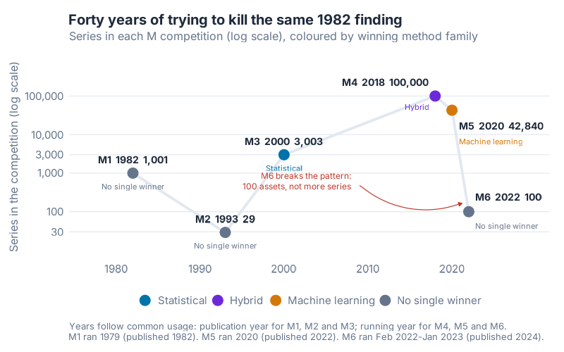
What jumped out at me plotting this is the last point. Every competition got bigger until M6, which shrank to 100 assets and asked a different question entirely. More on that at the end.

1982: the finding that refused to die

M1 covered 1,001 series and 24 methods, counting variations. It produced three conclusions, and forecasting has been arguing with all three ever since.

Statistically sophisticated methods did not beat simpler ones. Combinations of methods beat their own members. And the ranking of methods changed depending on which error measure you used and how far ahead you looked.

That third finding is the awkward one. It means "which model is best" is not a well-posed question until you have named your metric and your horizon. Most model bake-offs skip that step entirely.

1993: so they blamed the humans

The natural objection to M1 is that the competition was rigged against expertise. No human was allowed to look at a series and apply what they knew about the business behind it. Strip out judgment and of course the plain formulas do fine.

M2 was built to test exactly that. It ran in real time on 29 series, 23 from four companies and 6 macroeconomic, with five human forecasters working alongside the automatic methods. These were method experts recruited through a journal announcement, not company planners. The access was contractual. Companies agreed to hand over whatever extra information the forecasters asked for, and the whole exercise ran twice over four years.

Judgment got every advantage the format allowed. It did not improve on the pure statistical methods. The paper’s own words: "forecasters did not improve the accuracy of mechanical methods."

This is the M-competition result I see inverted most often, and I had it inverted myself until I read the paper. M2’s design reads like its conclusion. Give forecasters context and let them override, and surely the numbers improve. They didn’t.

M2 is also the weakest of the six as evidence, and I would rather say so than lean on it. Twenty-nine series is a small sample. Hyndman has argued that few general conclusions can be drawn at that size, and he is right. Treat it as one failed attempt to rescue the 1982 result, not as proof that judgment never helps.

M2 also complicates the 1982 combination result, which is worth flagging rather than hiding. Its most accurate method was damped trend exponential smoothing. A combination of smoothing methods came second, close behind. The paper’s verdict on combining: it "does not beat the best of the individual smoothing methods but does well on average."

Hold onto that. It comes back when I run the experiment myself.

2000: the winner was a formula in a costume

M3 was the big replication: 3,003 series, 24 methods, five different accuracy measures reported side by side.

The Theta method came out on top on the competition’s headline accuracy measure. I am being careful with that phrasing on purpose. M3 crowned no single prize winner, and one of its own published findings is that rankings shift as you change the measure. Anyone who tells you a method flatly "won M3" has skipped the paper’s most useful caveat.

The other M3 result deserves more attention than it gets. Brown’s Single Exponential Smoothing and Gardner’s Damped Trend, two methods built by working forecasters rather than theorists, did as well as and in many cases better than ARIMA and ARARMA. Damped trend in particular has been quietly winning arguments ever since. It was already the single most accurate method on M2’s series in 1993, and six years after M3 it was the bar in NN3 that exactly one neural network managed to clear.

And then Hyndman and Billah pulled the costume off the winner.

Interlude, 2006: neural networks get a fair fight

By the mid-2000s the neural network community had a reasonable complaint. M3 was not designed for them, and a competition’s format shapes who can win it.

So NN3 was built on M3 data to give neural networks and computational-intelligence methods their shot. It drew 59 submissions. That made it the largest such competition on time series data at that point.

Exactly one neural network beat the damped trend benchmark on sMAPE. The best overall result came from a novel statistical method, which outperformed all of the statistical and computational-intelligence benchmarks.

Now the detail that makes it sharper, and that I got wrong before checking. Only computational-intelligence entries could win. The lowest error in the whole competition belonged to a statistical method that was not eligible for the prize. The official winner, an echo state network, came third on raw error. Second was the Theta method. It was there as a benchmark. The formula Hyndman and Billah had unmasked five years earlier beat the neural network that won.

So the competition built to showcase neural networks was topped by a statistical method it had disqualified in advance.

2018: eight point six percent

M4 changed the scale: 100,000 series, 61 methods, six sampling frequencies from yearly to hourly.

M4 scored entries with OWA, a blend of sMAPE and MASE, normalised so that the competition’s Naive2 benchmark sits at exactly 1.000. Lower is better. M4 also supplied a Comb benchmark: the equal-weight average of three exponential smoothing models, single, Holt and damped. It scored 0.898.

Sit with that benchmark for a second. It is the whole argument in one object: three textbook smoothing formulas, the newest of them from the 1980s, averaged with no weighting and nothing learned. All six pure machine learning methods entered in M4 failed to beat it. Not one got past the average.

Slawek Smyl won with 0.821.

Read those two numbers together. The winner, a hybrid neural network trained on a hundred thousand series, beat a plain average of textbook smoothing models by 8.6%. It won on merit. But 8.6% over a benchmark any competent analyst could build in an afternoon is not the margin the relay-race story implies.

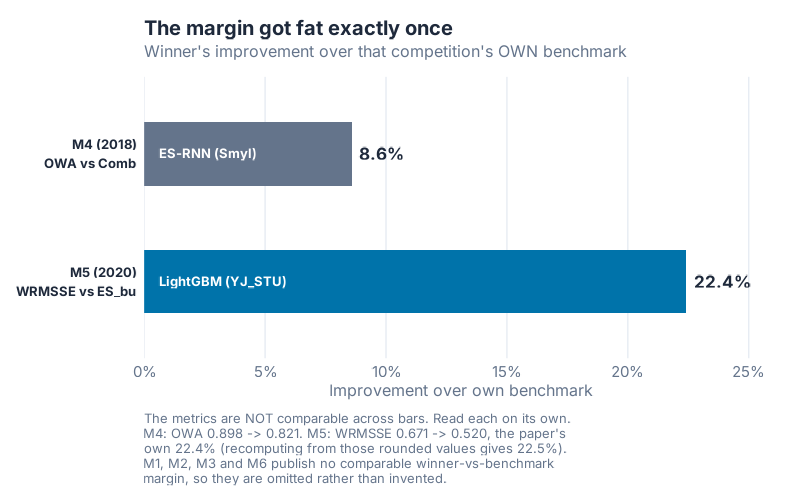
Only two competitions publish a clean winner-against-benchmark margin, so the chart has two bars. The metrics behind them measure different things on different data, so those two bars are not strictly comparable to each other either. Two honest bars beat six invented ones.

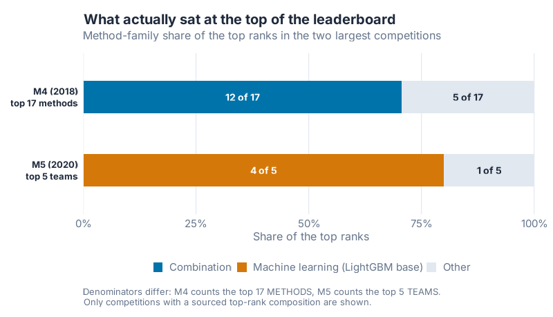
The composition of the leaderboard matters more than the winner. Of the 17 most accurate methods in M4, 12 were combinations. Six of the methods entered were pure machine learning, and only one of those beat Naive2. Not the Comb benchmark. Naive2.

Two details about M4 get mangled constantly, so let me be specific.

Smyl’s winner is usually described as a neural network. It is better described as exponential smoothing and a neural network welded together. Each series gets its own level and seasonal smoothing parameters, and those are learned jointly with dilated-LSTM stacks whose weights are global, shared across series rather than fitted per series. Deseasonalisation happens inside the model rather than as a preprocessing step. The per-series half handles level and season, the global half learns the shape that many series share. There is no trend term.

Second place gets mangled even more often, and this one is worth watching closely because of who mangled it. Second place, at OWA 0.838, was FFORMA. It pools nine forecasting methods, eight statistical plus one neural network, then uses XGBoost to learn the averaging weights from features of each series. XGBoost never forecasts anything. It decides how much to trust each classical model on each series.

So FFORMA is a combination method wearing a machine learning hat, and describing it as an XGBoost forecaster inverts what M4 demonstrated. Now the part I enjoy: the M4 organisers’ own findings paper describes it as "a combination of seven statistical methods and one ML one." Seven plus one is eight. FFORMA’s authors say nine, in their own paper and in their own published code. The people running the competition miscounted the runner-up’s ingredients, and the secondary literature has been copying that miscount ever since.

2020: machine learning finally wins, and why

Then M5 broke the pattern, and it broke it cleanly.

M5 used 42,840 hierarchical Walmart series, five years of daily history, a 28-day horizon. The winner, competing solo, scored a WRMSSE of 0.520 against the best statistical benchmark at 0.671. That is the 22.4% the organisers report, computed before those figures were rounded to three decimals. Divide the rounded pair yourself and you get 22.5%. It cost 220 LightGBM models at six per series. Four of the top five teams used LightGBM. Machine learning did not squeak past the benchmark, it walked past it. I covered the full M5 result separately, including why a shallow neural net still lost to seasonal naive.

But that 22.4% is an average across all twelve of M5’s aggregation levels, and the levels tell different stories.

At Level 1, total sales across the chain, the winner scored 0.199 against the benchmark’s 0.426. A 53.3% improvement. At Level 12, a single product in a single store, the level your ERP and MRP actually plan against, the winner scored 0.884 against 0.915. A 3.39% improvement.

So the one unambiguous machine learning victory in forty years of competitions is worth 53.3% where nobody makes replenishment decisions and 3.39% where everybody does.

Here’s my read on why M5 went the other way. It isn’t the algorithms. M5 handed competitors price, promotions, calendar events and SNAP benefit timing. Every earlier competition handed over a bare series and nothing else. Gradient boosting is a machine for exploiting covariates, and M5 was the first competition to supply any. The data got richer. The models just got to use it.

Every winner was unusable

Line the champions up and something awkward becomes obvious.

The M5 winner is 220 gradient-boosted models, six per series. The M4 winner needs a GPU and builds a different computational graph for every series it fits. The M4 runner-up is a meta-learner sitting on top of nine other models. Now picture any of that in your planning stack. None of it survives contact with a system that has to run overnight, every night, and be debuggable by whoever is on call.

What actually made it into daily practice came from further down the leaderboard. Combine your models. Damp your trends. Deseasonalise before you fit. Every one of those ideas is cheap, boring, decades old, and has been in the top ten of these competitions since 1982.

The 1982 finding, on data you can pull in three lines

The claim I find most useful from all six competitions is also the easiest to test yourself: a plain average of several models beats the models it averages. So I tested it.

I reused the data and the scoring code from an earlier race against Amazon’s forecasting AI: 148 Australian retail turnover series, training data through December 2016, a 24-month test window, scored with MASE. Reusing it matters, because the new numbers then have to reproduce the published ones. They do, to within 0.0033. If they hadn’t, nothing below would be worth reading.

Five members in the pool: ETS, ARIMA, STL-ETS, Theta (the method that topped M3’s headline measure, so it seemed rude to leave it out) and seasonal naive. Then I scored all 31 possible equal-weight combinations.

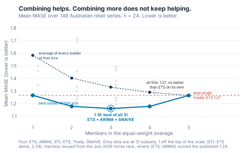
The best single model was ETS at 1.2667. The best combination was ETS plus ARIMA plus seasonal naive at 1.1615, an 8.3% improvement. Averaging in a free, one-line baseline made the pair of trained models better. That is the 1982 finding, reproduced on public data, in 2026.

Now the part I did not expect. The curve turns around. Four members scored 1.1788 and all five scored 1.2656, barely distinguishable from ETS on its own. Adding members stops helping and starts hurting.

The culprit is STL-ETS at 2.3440. It is dismal, and any subset containing it inherits the damage. So combination is not a free lunch you can order more of. It cancels uncorrelated errors between models that are each individually credible, and one bad member poisons the average.

I ran the whole sweep again with a stronger STL-ETS, to check whether the shape was an artifact of one weak entry. The peak stayed at three members. That makes it a finding rather than a coincidence. (I am not treating that second run as the headline. The stronger variant is methodologically looser, because it lets ETS refit the seasonality STL was supposed to have removed already.)

One more number, because means flatter combinations. On a per-series basis, the three-model average beat ETS alone on 98 of the 148 series, or 66.2%. Two times in three, not always. Report that number and not just the average, or you are overselling.

2022: does a better forecast make you money?

M6 asked the question the previous five carefully avoided. Not "whose forecast is most accurate" but "does accuracy convert into a better decision."

The design is two races at once. 226 teams forecast 100 assets, 50 S&P 500 stocks and 50 international ETFs, over twelve monthly rounds. They were scored on forecast accuracy with a ranked probability score, and separately on investment return with an information ratio. Same teams, same twelve months, two independent scoreboards.

Across the teams whose forecasts differed from the benchmark, the correlation between forecasting accuracy and investment return was r = 0.04.

Nothing. Being right and making money were unrelated.

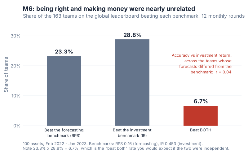
The beat-rates say it again. Of the 163 teams that entered at the start and made the global leaderboard, 23.3% beat the forecasting benchmark. 28.8% beat the investment benchmark. Only 6.7% beat both. Multiply the first two together and you get 6.7%, which is precisely the joint rate you would expect if forecasting skill and investment skill were statistically independent. Three of those teams beat the forecasting benchmark in all twelve months. None beat the investment benchmark all twelve.

And the finding that closes the loop back to 1982: averaging the forecasts of the top-performing teams beat every individual team in the competition.

Financial markets are not supply chains, and I won’t pretend the transfer is automatic. But the shape of the problem is the one in your S&OP meeting, and I have written before about forecasts that improve without improving anything downstream. M6 is the cleanest evidence I know that accuracy and outcome are separate variables. If your accuracy programme has never checked whether better numbers changed a single order quantity, M6 is your warning.

The strongest case against all of this

Two published objections deserve a hearing. Both come from inside the tent.

The first is statistical. M3’s conclusions rested on descriptive comparisons, with no significance testing behind them. In 2005 Koning, Franses, Hibon and Stekler applied formal multiple-comparison tests to the M3 results and reported that the claim a combination beats the methods being combined was not proven. Note the third author. Michèle Hibon co-organised M3, so one of the organisers co-authored the paper finding that their own competition’s conclusion did not hold up.

The second objection comes from Hyndman, in a published history of these competitions. On M3: Makridakis and Hibon "claimed that the M3 competition upheld the findings of their earlier work, yet the results did not provide the evidence supporting the first finding (that simple methods outperform more complicated methods)."

Look at M3’s top two and the objection lands. Theta only looked simple after Hyndman and Billah took it apart, which is the story this post opened with. The other was ForecastPro, a commercial package that picks between exponential smoothing and ARIMA using state-space approximations and a BIC calculation. Nobody would call that simple.

So the tidy version of the argument does not survive contact with its own literature. Good. It shouldn’t.

What survives is narrower and more useful to you. Combining helps, and it helps reliably, but it does not beat every member every time and it stops helping the moment you add a weak one. That is what my 148 series say. It is what M2’s own tables said in 1993. And it is the version Koning and colleagues never put to the test, because it is a claim about defaults rather than about winners. The sentence worth defending is not "combinations win." It is that a combination of individually decent models is the best default you can build in eight lines of code, and the competitions have never dislodged that.

Where this breaks

Three honest limits.

First, the M-competition archives are mostly aggregated and covariate-free. That favours simple methods structurally, because there is nothing else in the data for a complex model to find. M5 is the proof. Hand over promotions and prices, and gradient boosting pulls ahead. If your data is rich, the pre-M5 results understate what machine learning can do for you.

Second, the margins are measured in different currencies. M3 reported five accuracy measures, M4 used OWA, M5 used WRMSSE, M6 used a ranked probability score. Read each bar on its own, never as a trend line.

Third, my combination test runs on 148 aggregated Australian retail series with decades of clean monthly history. That is a long way from an intermittent spare part with eleven sales in two years. My hunch is that combination still helps there and the leaderboard compresses hard. But I have not tested it. A hunch is not a result.

Your next steps this week

1. Average your two best models and score the result. Not a weighted blend, not a meta-learner. The arithmetic mean. On this data, averaging ETS and ARIMA scored 1.2367 against 1.2667 for ETS alone.
2. Then add seasonal naive to that average. The free one-line baseline pulled the same combination to 1.1615: 8.3% better than the best single model, 6.1% better than the trained pair. Score it per series as well, because a mean can hide a model that wins big twice and loses small forty times. Here the three-model average won on 98 of 148.
3. Score your forecast at the granularity you actually order at. Aggregate accuracy is the number that flatters everyone. M5’s winner was worth 53.3% at chain level and 3.39% at SKU-store. Only one of those numbers touches a purchase order.
4. Score every member alone, then drop your worst one and re-score. Four members beat five on my data, and the one I removed was the member that scored worst by itself. Do it in that order. Dropping a good model will make things worse and teach you nothing.
5. Take one accuracy claim into your next S&OP meeting and ask what decision it changed. Not what the MAPE was. What got ordered differently. Expect the room to struggle with the question. That struggle is the useful part, and it is the M6 result arriving in your own building.

source("Scripts/theme_inphronesys.R")
suppressPackageStartupMessages({
  library(fpp3); library(dplyr); library(tidyr); library(purrr); library(readr)
})

M <- 12L   # monthly seasonal period
H <- 24L   # forecast horizon

# --- MASE, identical to Scripts/horserace/score_horserace.R -------------------
#   scale = mean_{t=m+1..n} |Y_t - Y_{t-m}|  on TRAIN
#   MASE  = mean_h |actual_h - forecast_h| / scale     (per series)
#   report = mean MASE across the 148 series
scales_tbl <- train_raw |>
  arrange(series_id, month) |>
  group_by(series_id) |>
  summarise(mae_scale = mean(abs(turnover - lag(turnover, M)), na.rm = TRUE),
            .groups = "drop")
stopifnot(all(scales_tbl$mae_scale > 0))

# One fixed row ordering shared by the actuals and every forecast column.
key <- test_raw |>
  arrange(series_id, month) |>
  rename(actual = turnover) |>
  left_join(scales_tbl, by = "series_id")
stopifnot(nrow(key) == 3552L, !anyNA(key$mae_scale))

mase_per_series <- function(fvec) {
  tibble(series_id = key$series_id,
         abs_err   = abs(key$actual - fvec),
         mae_scale = key$mae_scale) |>
    group_by(series_id) |>
    summarise(mase = mean(abs_err) / first(mae_scale), .groups = "drop")
}
mean_mase <- function(fvec) mean(mase_per_series(fvec)$mase)

# --- The two new members -----------------------------------------------------
# STL then ETS(A,A,N) on the seasonally adjusted series, matching the spec used
# in the earlier six-model post.
stl_ets_spec <- decomposition_model(
  STL(turnover ~ trend(window = 13) + season(window = "periodic"), robust = TRUE),
  ETS(season_adjust ~ error("A") + trend("A") + season("N"))
)

# No THETA() in core fable, so route forecast::thetaf through per-series ts
# objects. Every train series is contiguous monthly, so ts() is exact.
fit_theta <- function() {
  train_raw |>
    arrange(series_id, month) |>
    group_split(series_id) |>
    map_dfr(function(d) {
      st <- as.integer(strsplit(d$month[1], "-")[[1]])
      y  <- stats::ts(d$turnover, start = c(st[1], st[2]), frequency = M)
      tibble(series_id = d$series_id[1],
             month     = format(seq(as.Date("2017-01-01"), by = "month",
                                    length.out = H), "%Y-%m"),
             model     = "theta",
             forecast  = as.numeric(forecast::thetaf(y, h = H)$mean))
    })
}

# --- Equal-weight sweep over all 2^5 - 1 subsets ------------------------------
combine_equal <- function(Fmat, members) {
  if (length(members) == 1L) Fmat[, members]
  else rowMeans(Fmat[, members, drop = FALSE])
}

sweep_subsets <- function(members) {
  Fmat <- forecast_matrix(members)
  subs <- unlist(lapply(seq_along(members),
                        function(k) combn(members, k, simplify = FALSE)),
                 recursive = FALSE)
  stopifnot(length(subs) == 2^length(members) - 1L)
  map_dfr(subs, function(s) tibble(
    k         = length(s),
    members   = paste(s, collapse = "+"),
    mean_mase = mean_mase(combine_equal(Fmat, s))
  )) |> arrange(mean_mase)
}

MEMBERS <- c("ets", "arima", "stl_ets", "theta", "snaive")
subsets <- sweep_subsets(MEMBERS)

# --- Hard regression gate ----------------------------------------------------
# These four figures are already published. We rescore the SAME cached point
# forecasts through the SAME MASE path, so agreement must be near-exact.
gate <- tibble(
  members     = c("ets+arima", "ets", "arima", "snaive"),
  published_v = c(1.24, 1.27, 1.35, 1.46)
) |>
  left_join(subsets |> select(members, mean_mase), by = "members") |>
  mutate(d    = round(mean_mase - published_v, 4),
         flag = ifelse(abs(d) > 0.02, "CHECK", "ok"))

if (!all(gate$flag == "ok")) {
  stop("REGRESSION GATE FAILED - harness reuse is broken. Not producing charts.")
}

References

• Makridakis, S., Andersen, A., Carbone, R., Fildes, R., Hibon, M., Lewandowski, R., Newton, J., Parzen, E., & Winkler, R. (1982). The accuracy of extrapolation (time series) methods: Results of a forecasting competition. Journal of Forecasting, 1(2), 111-153. https://doi.org/10.1002/for.3980010202
• Makridakis, S., et al. (1993). The M2-competition: A real-time judgmentally based forecasting study. International Journal of Forecasting, 9(1), 5-22.
• Makridakis, S., & Hibon, M. (2000). The M3-Competition: results, conclusions and implications. International Journal of Forecasting, 16(4), 451-476. https://doi.org/10.1016/S0169-2070(00)00057-1
• Assimakopoulos, V., & Nikolopoulos, K. (2000). The theta model: a decomposition approach to forecasting. International Journal of Forecasting, 16(4), 521-530.
• Hyndman, R. J., & Billah, B. (2003). Unmasking the Theta method. International Journal of Forecasting, 19(2), 287-290. DOI: 10.1016/S0169-2070(01)00143-1. Preprint dated 27 September 2001: https://robjhyndman.com/papers/Theta.pdf
• Crone, S. F., Hibon, M., & Nikolopoulos, K. (2011). Advances in forecasting with neural networks? Empirical evidence from the NN3 competition on time series prediction. International Journal of Forecasting, 27(3), 635-660. https://doi.org/10.1016/j.ijforecast.2011.04.001
• Makridakis, S., Spiliotis, E., & Assimakopoulos, V. (2020). The M4 Competition: 100,000 time series and 61 forecasting methods. International Journal of Forecasting, 36(1), 54-74. https://doi.org/10.1016/j.ijforecast.2019.04.014
• Makridakis, S., Spiliotis, E., & Assimakopoulos, V. (2018). The M4 Competition: Results, findings, conclusion and way forward. International Journal of Forecasting, 34(4), 802-808. https://doi.org/10.1016/j.ijforecast.2018.06.001. The source of the "seven statistical methods and one ML one" description of FFORMA quoted above.
• Montero-Manso, P., Athanasopoulos, G., Hyndman, R. J., & Talagala, T. S. (2020). FFORMA: Feature-based forecast model averaging. International Journal of Forecasting, 36(1), 86-92. https://doi.org/10.1016/j.ijforecast.2019.02.011
• Smyl, S. (2020). A hybrid method of exponential smoothing and recurrent neural networks for time series forecasting. International Journal of Forecasting, 36(1), 75-85. DOI: 10.1016/j.ijforecast.2019.03.017. The ES-RNN method paper, and the source for the architecture description above.
• Smyl, S. M4 Forecasting Competition: Introducing a New Hybrid ES-RNN Model. Uber Engineering. https://www.uber.com/blog/m4-forecasting-competition/
• Crone, S. F., Hibon, M., & Nikolopoulos, K. (2011). Advances in forecasting with neural networks? Empirical evidence from the NN3 competition on time series prediction. International Journal of Forecasting, 27(3), 635-660. DOI: 10.1016/j.ijforecast.2011.04.001
• Makridakis, S., Spiliotis, E., & Assimakopoulos, V. (2022). The M5 competition: Background, organization, and implementation. International Journal of Forecasting, 38(4). https://doi.org/10.1016/j.ijforecast.2021.07.007
• Makridakis, S., Spiliotis, E., & Assimakopoulos, V. (2022). M5 accuracy competition: Results, findings, and conclusions. International Journal of Forecasting, 38(4). https://doi.org/10.1016/j.ijforecast.2021.11.013
• Makridakis, S., Spiliotis, E., et al. (2024). The M6 forecasting competition: Bridging the gap between forecasting and investment decisions. International Journal of Forecasting. https://doi.org/10.1016/j.ijforecast.2024.05.007 (preprint: https://arxiv.org/abs/2310.13357)
• Koning, A. J., Franses, P. H., Hibon, M., & Stekler, H. O. (2005). The M3 competition: Statistical tests of the results. International Journal of Forecasting, 21(3), 397-409. https://doi.org/10.1016/j.ijforecast.2004.10.003. The formal significance tests M3’s own conclusions never ran.
• Hyndman, R. J. (2020). A brief history of forecasting competitions. International Journal of Forecasting, 36(1), 7-14. DOI: 10.1016/j.ijforecast.2019.03.015. Author’s accepted manuscript, which is the copy quoted here: https://robjhyndman.com/papers/forecasting-competitions.pdf. The source of the objection that M3 did not evidence its own simple-beats-complex finding.
• Gardner, E. S., Jr., & McKenzie, E. (1985). Forecasting trends in time series. Management Science, 31(10), 1237-1246. DOI: 10.1287/mnsc.31.10.1237. The damped trend method, and the newest of the three formulas in M4’s Comb benchmark.
• Hyndman, R. J., & Koehler, A. B. (2006). Another look at measures of forecast accuracy. International Journal of Forecasting. The source of MASE, the metric used throughout the combination test above.
• Australian Bureau of Statistics retail turnover, monthly, distributed as aus_retail in the tsibbledata R package. https://tsibbledata.tidyverts.org/