"Mercenaries and auxiliaries are useless and dangerous." That is Machiavelli’s verdict in Chapter 12 of The Prince (1513), and five centuries later the argument has aged better than the chapters around it. The case is structural, not moral. A hired soldier rationally minimises personal risk at the moment of greatest stress. So does a hired strategist. So does a contract engineer at the core of a delivery team. The incentive reverses exactly when you need it not to.
The Argument in Chapter 12
Machiavelli’s catalogue is direct. Mercenary armies are, in W. K. Marriott’s translation, "disunited, ambitious, and without discipline, unfaithful, valiant before friends, cowardly before enemies." (Machiavelli, The Prince, Ch. 12, trans. W. K. Marriott, 1908; Project Gutenberg eBook 1232.) The diagnosis. They fight when fighting is cheap and run when it is not. They have no homeland to defend, no covenant with the city, and no career consequence that outlasts the campaign. In peacetime they bleed the treasury. In war they bleed the prince.
What carries the argument across five centuries is not the era’s contempt for hired troops. It is the incentive structure. The captain paid by the month earns more by extending the war, less by ending it, and nothing at all by dying for the cause. The principal’s downside does not flow to the agent, so the agent allocates effort to whatever does.
The Strategy-Consultant Problem
Lift that structure out of 1513 and drop it into a modern transformation programme. The shape repeats.
A consultancy is paid to produce the deck, the model, the implementation plan. The engagement ends. Accountability for the operating consequence ends with it. Whatever the engagement team learned during eighteen months of work walks out of the building with them, because the firm bought exposure to a capability rather than the capability itself. The arrangement is fine for one-off questions where the answer is the deliverable. It breaks the moment the capability becomes part of how the firm runs.
The math is the surprise. The financial case for the alternative tends to land hardest with people who haven’t run it.
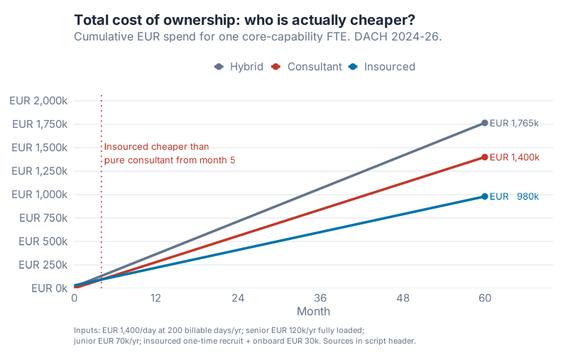
Set the inputs first. Senior consulting day rate of €1,400, sitting between the BDU’s 2025 industry-survey average of €1,300 and the partner-band figure of €1,600 for senior management consulting in Germany (BDU, Studie Honorare im Consulting 2025), at 200 billable days a year. Senior internal fully loaded: €120,000 a year. Junior: €70,000. A one-time €30,000 to recruit and onboard the team.
Run the model out 60 months. Pure consultant: €1,400,000. Hybrid: €1,765,000. Insourced: €980,000. Insourced becomes cheaper than pure consultant from month 5 onward. Five-year savings: €420,000 against pure consultant (30.0%) and €785,000 against hybrid (44.5%). The arithmetic isn’t subtle. The reason most firms still pay it is that the consulting line and the headcount line live in different parts of the budget, and a CFO with a hiring freeze still has the discretion to sign a statement of work.
The Capability Cliff
What the TCO chart understates is the asset side. Money paid to a consultant is money. Money paid to an employee is money plus an accumulating stock of knowledge that stays with you.
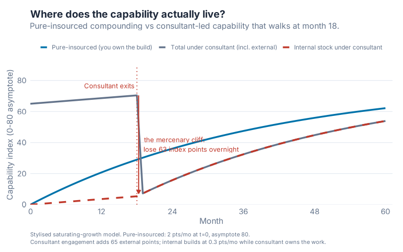
The consultant-led line in this stylised model climbs to a total of 70.4 capability index points by month 18, because the consultant brings external expertise on top of the firm’s slow internal build. At month 19 the engagement ends. Total capability collapses to 7.2 the next month. A drop of 63.2 points overnight. That is the mercenary cliff. The internal team, whose own stock at month 18 had only reached 5.4 because the consultant owned the decisions, then begins a real build from a low base. After three and a half more years of rebuild, internal capability reaches 53.9. An alternate timeline that insourced from day one reaches 62.1 in the same window. Forty-two months after the consultant exit, the firm is still 8.3 points behind where it would have been if it had built the team itself.
Cash is one cost. The option you didn’t buy is the other.
The Gig and Platform Parallel
The same structural problem appears whenever a firm puts contracted labour at the operational core rather than the periphery. Drivers, riders, contract engineers, gig-platform agents who interact with the customer. The work is the firm’s product. The workers are structurally external. When demand spikes, when a regulator surprises, when a competitor undercuts the price floor, the workforce is contractually free to disappear. Machiavelli would recognise the position. The army the prince has hired is loyal until the contract ends. The contract ends when the prince needs it not to.
Whose Effort Goes Up When the Project Catches Fire
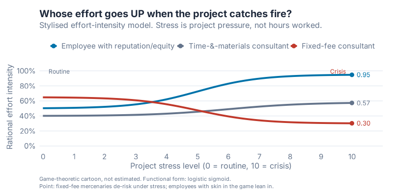
The chart caption says it plainly. The point it makes is the one Machiavelli made. Under low project stress, a fixed-fee consultant is the most active actor on the chart (0.65), the employee sits in the middle (0.50), and a time-and-materials consultant is the least active (0.40). Push the project into crisis and the ranking flips. Fixed-fee effort falls to 0.30. Time-and-materials drifts up to 0.57. The employee, whose reputation and bonus and continued employment depend on the outcome, climbs to 0.95. At crisis the employee runs at roughly three times the fixed-fee consultant’s effort. That is Machiavelli’s structural claim translated into a single ratio.
Citizen Armies and the Toyota Alternative
Chapter 13 is the constructive half. The remedy for mercenary failure is to build your own forces, train them yourself, and accept the cost. Chapter 14 extends the argument into peacetime: the prince should study war, terrain, and history when no campaign is on the calendar, because skill that rusts between conflicts loses the next one. (Machiavelli, The Prince, Ch. 13 and Ch. 14.)
The modern instance every operations reader will recognise is the Toyota Production System. Jeffrey K. Liker, The Toyota Way (McGraw-Hill, 2004; second edition 2020). The system treats line workers as engineers. Process improvement is owned by the people who do the work, not by an external transformation team that runs a kaizen event and leaves. The capability compounds because it lives inside the people the firm doesn’t lay off.
The mechanism is not romantic. Insourcing is more expensive in month one. It pays back in the capability that accumulates between month one and month sixty.
When Mercenaries Are the Right Call
The honest counterpoint. Not all work is core. A firm that insources its window cleaning, its tax filing, and its commodity legal review is wasting money it could spend on the work that actually distinguishes it. The distinction Machiavelli pressed in 1513 is the same one to press now. Hire for the periphery. Build for the core.
I think most senior teams know this in the abstract and lose it in the quarter. The discipline is in two parts. Know which work is core. Re-classify on the day a function becomes strategic, and insource that day. The day you can’t run without a capability is the day you stop renting it.
Tomorrow the series stays with Machiavelli. Chapter 18 of The Prince is the one quoted out of context more than any other: the fox and the lion, and the prince who needs both.
Friday, Article 13: "Of the Fox and the Lion." Machiavelli on adaptive leadership.
Interactive Dashboard
Slide the day rate, the salary bands, and the engagement length. Watch the TCO crossover move and the capability cliff change shape.
Interactive Dashboard
Explore the data yourself — adjust parameters and see the results update in real time.
Show R Code
# =============================================================================
# generate_merc_images.R
# Charts for: "Mercenaries Will Ruin You: Machiavelli on Outsourced Core
#              Capability" (inphronesys.com, May 21, 2026)
# =============================================================================
# Three pedagogical / stylised models illustrating Machiavelli's argument in
# The Prince, chs. 12-14 that mercenary forces (here: pure-consultant or
# heavy-consultant operating models for CORE capability work) fail because
# incentives reverse under pressure. None of these are estimated from a
# proprietary dataset. They are transparent toy models with stated inputs.
#
# CITED INPUTS (real benchmarks, not invented):
#   - German consulting day rate, 2025: average invoiced EUR 1,300/day; partner
#     / executive tier EUR 1,600/day; analyst tier EUR 700/day. We use
#     EUR 1,400/day as a "senior tier-2" midpoint between the average and the
#     partner band. Verified URLs (page-fetched 2026-05-20):
#       BDU "Studie Honorare im Consulting 2025"  https://www.bdu.de/news/studie-honorare-im-consulting-2025-tagessaetze-leicht-ruecklaeufig/
#         (primary; quotes: "Der durchschnittlich fakturierte Tagessatz
#          betraegt 1.300 Euro in 2025"; "der Tagessatz eines
#          Geschaeftsfuehrers oder Partners im Durchschnitt bei 1.600 Euro";
#          "der eines Analysten bei 700 Euro".)
#       CONSULTING.de coverage of the same BDU study  https://www.consulting.de/artikel/ruecklaeufige-tagessaetze-im-consulting/
#         (corroborating, German trade press).
#   - Fully-loaded employer cost factor ~ 1.20-1.30 of gross salary for pure
#     Lohnnebenkosten; 1.50-1.65 once workplace, equipment, admin overhead are
#     included.
#       Sources:
#         Personio "Lohnnebenkosten"  https://www.personio.de/hr-lexikon/lohnnebenkosten/
#         Steuertipps Arbeitgeber-Brutto-Netto-Rechner  https://www.steuertipps.de/service/rechner/brutto-netto-gehaltsrechner-arbeitgeber
#       Senior fully-loaded EUR 120k/yr = EUR ~75k gross x ~1.60.
#       Junior fully-loaded EUR  70k/yr = EUR ~45k gross x ~1.55.
#
# PEDAGOGICAL INPUTS (illustrative, stated openly in the article):
#   - Capability stock growth rate, asymptote, atrophy fraction.
#   - Effort-vs-stress sigmoid parameters.
#   - One-time recruiting+onboarding spend.
# =============================================================================

suppressPackageStartupMessages({
  library(ggplot2)
  library(dplyr)
  library(tidyr)
  library(scales)
})

source("Scripts/theme_inphronesys.R")

img_dir <- "Images"
if (!dir.exists(img_dir)) dir.create(img_dir, recursive = TRUE)

# =============================================================================
# CHART 1 -- merc_tco_crossover.png
# 60-month cumulative TCO for three staffing modes
# =============================================================================

# --- Assumptions (cited above) -----------------------------------------------
day_rate        <- 1400          # EUR / billable consultant day
billable_days   <- 200           # billable consultant days per year
sen_loaded      <- 120000        # EUR / yr senior internal fully loaded
jun_loaded      <-  70000        # EUR / yr junior internal fully loaded
recruit_full    <-  30000        # one-time recruiting + onboarding (insourced)
recruit_hybrid  <-  15000        # one-time recruiting (hybrid - junior only)

# --- Monthly cash flow -------------------------------------------------------
months <- 0:60

consultant_per_mo <- day_rate * billable_days / 12        # ~ 23,333
hybrid_per_mo     <- consultant_per_mo + jun_loaded / 12  # ~ 29,167
insourced_per_mo  <- (sen_loaded + jun_loaded) / 12       # ~ 15,833

tco <- tibble(
  month = months,
  Consultant = consultant_per_mo * month,
  Hybrid     = recruit_hybrid + hybrid_per_mo * month,
  Insourced  = recruit_full   + insourced_per_mo * month
)

# --- Find crossover months (analytic) ----------------------------------------
# Insourced beats Consultant when:
#   recruit_full + insourced_per_mo * m  <  consultant_per_mo * m
#   m > recruit_full / (consultant_per_mo - insourced_per_mo)
cx_cons <- recruit_full / (consultant_per_mo - insourced_per_mo)
# Insourced beats Hybrid:
cx_hyb  <- (recruit_full - recruit_hybrid) / (hybrid_per_mo - insourced_per_mo)
cat(sprintf("Crossover insourced<consultant : month %.2f\n", cx_cons))
cat(sprintf("Crossover insourced<hybrid     : month %.2f\n", cx_hyb))

tco_long <- tco %>%
  pivot_longer(-month, names_to = "Mode", values_to = "EUR") %>%
  mutate(Mode = factor(Mode, levels = c("Hybrid", "Consultant", "Insourced")))

mode_colors <- c(
  "Insourced"  = iph_colors$blue,
  "Consultant" = iph_colors$red,
  "Hybrid"     = iph_colors$grey
)

# 5-yr endpoints for annotation
end5 <- tco_long %>% filter(month == 60)
cat("5-year cumulative TCO:\n")
print(end5)

p1 <- ggplot(tco_long, aes(x = month, y = EUR, color = Mode)) +
  geom_line(linewidth = 1.2) +
  geom_vline(xintercept = cx_cons, linetype = "dotted",
             color = iph_colors$red, linewidth = 0.6) +
  # NOTE: at the exact crossover month (cx_cons = 4.0) insourced and consultant
  # are equal; insourced is strictly cheaper only from the NEXT whole month
  # onward. Use floor(cx_cons) + 1, not ceiling(), to avoid labelling the
  # boundary month itself.
  annotate("text",
           x = cx_cons + 0.5, y = 1.55e6,
           label = sprintf("Insourced cheaper than\npure consultant from month %.0f",
                           floor(cx_cons) + 1),
           hjust = 0, vjust = 1, size = 3.4,
           color = iph_colors$red, family = "Inter") +
  # endpoint labels
  geom_point(data = end5, aes(x = month, y = EUR), size = 2.4) +
  geom_text(data = end5,
            aes(x = month + 0.8, y = EUR,
                label = paste0("EUR ", format(round(EUR / 1000), big.mark = ","), "k")),
            hjust = 0, vjust = 0.5, size = 3.4,
            family = "Inter", show.legend = FALSE) +
  scale_color_manual(values = mode_colors) +
  scale_y_continuous(
    labels = label_number(prefix = "EUR ", scale = 1e-3, suffix = "k", big.mark = ","),
    breaks = seq(0, 2e6, by = 250000),
    limits = c(0, 2.1e6),
    expand = expansion(mult = c(0, 0))
  ) +
  scale_x_continuous(breaks = seq(0, 60, by = 12),
                     limits = c(0, 70),
                     expand = expansion(mult = c(0, 0))) +
  labs(
    title = "Total cost of ownership: who is actually cheaper over 5 years?",
    subtitle = "Cumulative EUR spend for one core-capability FTE-equivalent. DACH benchmarks, 2024-2026.",
    x = "Month",
    y = NULL,
    color = NULL,
    caption = "Inputs: day rate EUR 1,400 (200 billable days/yr); senior fully-loaded EUR 120k/yr; junior EUR 70k/yr; insourced one-time recruit+onboard EUR 30k. Sources cited in script header."
  ) +
  theme_inphronesys(grid = "y") +
  theme(legend.position = "top",
        plot.caption = element_text(size = 9, color = iph_colors$grey,
                                     hjust = 0, margin = margin(t = 10)))

ggsave(file.path(img_dir, "merc_tco_crossover.png"), p1,
       width = 8, height = 5, dpi = 100, bg = "white")
cat("Saved: https://inphronesys.com/wp-content/uploads/2026/05/merc_tco_crossover-2.png\n")


# =============================================================================
# CHART 2 -- merc_capability_stock.png
# Capability stock under three operating models
# =============================================================================
#
# Pedagogical capability index. Asymptote = 80. Logistic-like saturating curve.
#   C(t) = K * (1 - exp(-k * t))
# k chosen so initial slope ~ 2 index-points / month for an insourced team
# (K*k = slope at t=0 -> k = 2/80 = 0.025).
#
# Consultant scenario:
#   - During engagement (months 0-18) the consultant provides an EXTERNAL stock
#     of 65 points on top of a tiny internal build of 0.3 pts/month (the
#     internal team does not have to own decisions).
#   - At month 18 the consultant exits and the external stock vanishes.
#   - Internal capability resumes building from a low base. The team has been
#     habituated to NOT owning the work, so the rebuild starts from the small
#     internal-only baseline.

months_cap <- 0:60
K   <- 80
k_r <- 0.025
engagement_end <- 18

internal_pure <- K * (1 - exp(-k_r * months_cap))                 # smooth

# Consultant scenario - internal-only stock
#   slow build during engagement, normal build after
internal_only_under_consultant <- numeric(length(months_cap))
slow_rate <- 0.3
for (i in seq_along(months_cap)) {
  t <- months_cap[i]
  if (t <= engagement_end) {
    internal_only_under_consultant[i] <- slow_rate * t
  } else {
    # Build from the level at month 18 using the same saturating curve, by
    # finding the effective time offset that matches starting level.
    start_lvl <- slow_rate * engagement_end
    delta_t   <- -log(1 - start_lvl / K) / k_r
    internal_only_under_consultant[i] <- K * (1 - exp(-k_r * (t - engagement_end + delta_t)))
  }
}

# Total capability under consultant (external boost only during engagement)
external_boost <- 65
total_under_consultant <- internal_only_under_consultant +
  ifelse(months_cap <= engagement_end, external_boost, 0)

cap_df <- tibble(
  month = months_cap,
  `Pure-insourced (you own the build)`     = internal_pure,
  `Total under consultant (incl. external)` = total_under_consultant,
  `Internal stock under consultant`         = internal_only_under_consultant
) %>%
  pivot_longer(-month, names_to = "Scenario", values_to = "Capability") %>%
  mutate(Scenario = factor(Scenario, levels = c(
    "Pure-insourced (you own the build)",
    "Total under consultant (incl. external)",
    "Internal stock under consultant"
  )))

cap_colors <- c(
  "Pure-insourced (you own the build)"      = iph_colors$blue,
  "Total under consultant (incl. external)" = iph_colors$grey,
  "Internal stock under consultant"         = iph_colors$red
)

cap_ltype <- c(
  "Pure-insourced (you own the build)"      = "solid",
  "Total under consultant (incl. external)" = "solid",
  "Internal stock under consultant"         = "dashed"
)

# Reporting numbers
report_pts <- cap_df %>%
  filter(month %in% c(0, 17, 18, 19, 60)) %>%
  arrange(Scenario, month)
cat("\nCapability stock checkpoints:\n")
print(report_pts)

cliff_drop <- total_under_consultant[months_cap == 18] -
              total_under_consultant[months_cap == 19]
cat(sprintf("Cliff drop month 18 -> 19 (consultant exit): %.1f index points\n",
            cliff_drop))

p2 <- ggplot(cap_df, aes(x = month, y = Capability,
                          color = Scenario, linetype = Scenario)) +
  geom_line(linewidth = 1.2) +
  geom_vline(xintercept = engagement_end, linetype = "dotted",
             color = iph_colors$red, linewidth = 0.6) +
  annotate("rect", xmin = engagement_end - 0.05, xmax = engagement_end + 0.05,
           ymin = 0, ymax = 80, alpha = 0) +
  annotate("text", x = engagement_end - 0.4,
           y = 78, label = "Consultant exits",
           hjust = 1, vjust = 1, size = 3.4,
           color = iph_colors$red, family = "Inter") +
  annotate("segment",
           x = engagement_end + 0.3, xend = engagement_end + 0.3,
           y = total_under_consultant[months_cap == 18],
           yend = total_under_consultant[months_cap == 19],
           arrow = arrow(length = unit(0.18, "cm"), type = "closed"),
           color = iph_colors$red, linewidth = 0.7) +
  annotate("text", x = engagement_end + 1.2,
           y = (total_under_consultant[months_cap == 18] +
                total_under_consultant[months_cap == 19]) / 2,
           label = sprintf("the mercenary cliff:\nlose %.0f index points overnight", cliff_drop),
           hjust = 0, vjust = 0.5, size = 3.4,
           color = iph_colors$red, family = "Inter") +
  scale_color_manual(values = cap_colors) +
  scale_linetype_manual(values = cap_ltype) +
  scale_y_continuous(limits = c(0, 90),
                     breaks = seq(0, 80, by = 20),
                     expand = expansion(mult = c(0, 0))) +
  scale_x_continuous(breaks = seq(0, 60, by = 12),
                     expand = expansion(mult = c(0, 0.02))) +
  labs(
    title = "Where does the capability actually live?",
    subtitle = "Pedagogical model: pure-insourced compounding vs consultant-led capability that walks out the door at month 18.",
    x = "Month",
    y = "Capability index (0-80 asymptote)",
    color = NULL, linetype = NULL,
    caption = "Stylised saturating-growth model. Pure-insourced: dC/dt at t=0 = 2 pts/mo, asymptote 80. Consultant engagement adds 65 external points; internal team builds at 0.3 pts/mo while consultant owns the work."
  ) +
  theme_inphronesys(grid = "y") +
  theme(legend.position = "top",
        legend.text = element_text(size = 9),
        plot.caption = element_text(size = 9, color = iph_colors$grey,
                                     hjust = 0, margin = margin(t = 10)))

ggsave(file.path(img_dir, "merc_capability_stock.png"), p2,
       width = 8, height = 5, dpi = 100, bg = "white")
cat("Saved: https://inphronesys.com/wp-content/uploads/2026/05/merc_capability_stock-2.png\n")


# =============================================================================
# CHART 3 -- merc_effort_under_stress.png  (wide / short)
# Stylised game-theoretic effort intensity vs project stress level
# =============================================================================
#
# Cartoon model -- NOT estimated. Stress runs 0 (routine) .. 10 (full crisis).
# Effort intensity in [0, 1].
#
# Functional forms (logistic):
#   sigmoid(x, k, x0) = 1 / (1 + exp(-k * (x - x0)))
#
# Fixed-fee consultant : effort = 0.65 - 0.35 * sigmoid(s, k=1.0, x0=5)
#   (rational risk-minimisation as the project goes sideways; they don't get
#    paid more for blood)
# Time & materials consultant : effort = 0.40 + 0.18 * sigmoid(s, k=0.8, x0=6)
#   (some upside from billing more hours, but capped low; still bounded by
#    "next client matters more than this one")
# Internal with retention/equity stake : effort = 0.50 + 0.45 * sigmoid(s, k=1.0, x0=5)
#   (reputation, bonus, career upside hinge on outcome; effort rises with
#    stress)
# =============================================================================

sigmoid <- function(x, k, x0) 1 / (1 + exp(-k * (x - x0)))

stress <- seq(0, 10, by = 0.05)

eff_df <- tibble(
  stress = stress,
  `Fixed-fee consultant`            = 0.65 - 0.35 * sigmoid(stress, k = 1.0, x0 = 5),
  `Time-&-materials consultant`     = 0.40 + 0.18 * sigmoid(stress, k = 0.8, x0 = 6),
  `Employee with reputation/equity` = 0.50 + 0.45 * sigmoid(stress, k = 1.0, x0 = 5)
) %>%
  pivot_longer(-stress, names_to = "Actor", values_to = "Effort") %>%
  mutate(Actor = factor(Actor, levels = c(
    "Employee with reputation/equity",
    "Time-&-materials consultant",
    "Fixed-fee consultant"
  )))

actor_colors <- c(
  "Employee with reputation/equity" = iph_colors$blue,
  "Time-&-materials consultant"     = iph_colors$grey,
  "Fixed-fee consultant"            = iph_colors$red
)

# Endpoints for reporting
endpoints <- eff_df %>%
  filter(stress %in% c(0, 5, 10)) %>%
  arrange(Actor, stress)
cat("\nEffort intensity at stress = 0, 5, 10:\n")
print(endpoints)

label_pts <- eff_df %>%
  filter(stress == 10)

p3 <- ggplot(eff_df, aes(x = stress, y = Effort, color = Actor)) +
  geom_line(linewidth = 1.3) +
  geom_point(data = label_pts, size = 2.4) +
  geom_text(data = label_pts,
            aes(x = stress + 0.15, label = sprintf("%.2f", Effort)),
            hjust = 0, vjust = 0.5, size = 3.4,
            family = "Inter", show.legend = FALSE) +
  annotate("text", x = 0.2, y = 1.02,
           label = "Routine", hjust = 0, vjust = 1,
           color = iph_colors$grey, size = 3.2, family = "Inter") +
  annotate("text", x = 9.8, y = 1.02,
           label = "Crisis", hjust = 1, vjust = 1,
           color = iph_colors$red, size = 3.2, family = "Inter") +
  scale_color_manual(values = actor_colors) +
  scale_x_continuous(breaks = 0:10, limits = c(0, 11),
                     expand = expansion(mult = c(0.01, 0))) +
  scale_y_continuous(limits = c(0, 1.05),
                     breaks = seq(0, 1, by = 0.2),
                     labels = percent_format(accuracy = 1)) +
  labs(
    title = "Whose effort goes UP when the project catches fire?",
    subtitle = "Stylised effort-intensity model. Stress on the x-axis is project pressure, not hours worked.",
    x = "Project stress level (0 = routine, 10 = crisis)",
    y = "Rational effort intensity",
    color = NULL,
    caption = "Game-theoretic cartoon, not estimated parameters. Functional form: logistic sigmoid. Point: fixed-fee mercenaries de-risk under stress; employees with skin in the game lean in."
  ) +
  theme_inphronesys(grid = "y") +
  theme(legend.position = "top",
        plot.caption = element_text(size = 9, color = iph_colors$grey,
                                     hjust = 0, margin = margin(t = 10)))

ggsave(file.path(img_dir, "merc_effort_under_stress.png"), p3,
       width = 8, height = 4, dpi = 100, bg = "white")
cat("Saved: https://inphronesys.com/wp-content/uploads/2026/05/merc_effort_under_stress-2.png\n")


# =============================================================================
# DATASET SUMMARY (printed -- Alpha/Charlie copy these EXACT numbers)
# =============================================================================
cat("\n=============================================================\n")
cat("FINAL DATASET SUMMARY (Bravo-Zero-R -> Alpha-Zero-Blog/Charlie-Zero)\n")
cat("=============================================================\n")
cat("ASSUMPTIONS\n")
cat(sprintf("  day_rate              = EUR %s/day\n", format(day_rate, big.mark=",")))
cat(sprintf("  billable_days/yr      = %d\n", billable_days))
cat(sprintf("  senior fully loaded   = EUR %s/yr\n", format(sen_loaded, big.mark=",")))
cat(sprintf("  junior fully loaded   = EUR %s/yr\n", format(jun_loaded, big.mark=",")))
cat(sprintf("  recruit_full          = EUR %s one-time\n", format(recruit_full, big.mark=",")))
cat(sprintf("  recruit_hybrid        = EUR %s one-time\n", format(recruit_hybrid, big.mark=",")))
cat(sprintf("  engagement_end        = month %d\n", engagement_end))
cat(sprintf("  capability asymptote  = %d index pts\n", K))
cat(sprintf("  insourced growth rate = dC/dt at t=0 = %.2f pts/mo\n", K * k_r))
cat("\nCHART 1 -- TCO\n")
cat(sprintf("  60-mo TCO consultant : EUR %s\n",
            format(tco$Consultant[tco$month==60], big.mark=",")))
cat(sprintf("  60-mo TCO hybrid     : EUR %s\n",
            format(tco$Hybrid[tco$month==60], big.mark=",")))
cat(sprintf("  60-mo TCO insourced  : EUR %s\n",
            format(tco$Insourced[tco$month==60], big.mark=",")))
cat(sprintf("  crossover consultant : month %.2f\n", cx_cons))
cat(sprintf("  crossover hybrid     : month %.2f\n", cx_hyb))
cat(sprintf("  savings insourced vs consultant @ 60mo : EUR %s (%.1f%%)\n",
            format(tco$Consultant[tco$month==60] - tco$Insourced[tco$month==60],
                   big.mark=","),
            100 * (tco$Consultant[tco$month==60] -
                   tco$Insourced[tco$month==60]) /
                  tco$Consultant[tco$month==60]))
cat(sprintf("  savings insourced vs hybrid     @ 60mo : EUR %s (%.1f%%)\n",
            format(tco$Hybrid[tco$month==60] - tco$Insourced[tco$month==60],
                   big.mark=","),
            100 * (tco$Hybrid[tco$month==60] -
                   tco$Insourced[tco$month==60]) /
                  tco$Hybrid[tco$month==60]))
cat("\nCHART 2 -- CAPABILITY\n")
cat(sprintf("  pure-insourced @ mo60         : %.1f\n",
            internal_pure[months_cap == 60]))
cat(sprintf("  total under consultant @ mo17 : %.1f\n",
            total_under_consultant[months_cap == 17]))
cat(sprintf("  total under consultant @ mo18 : %.1f (last month with consultant)\n",
            total_under_consultant[months_cap == 18]))
cat(sprintf("  total under consultant @ mo19 : %.1f (mercenary cliff)\n",
            total_under_consultant[months_cap == 19]))
cat(sprintf("  internal stock @ mo60 (post-consultant rebuild) : %.1f\n",
            internal_only_under_consultant[months_cap == 60]))
cat(sprintf("  capability gap pure vs post-consultant @ mo60   : %.1f pts\n",
            internal_pure[months_cap == 60] -
              internal_only_under_consultant[months_cap == 60]))
cat("\nCHART 3 -- EFFORT vs STRESS\n")
ep_wide <- endpoints %>% pivot_wider(names_from = stress, values_from = Effort,
                                      names_prefix = "s")
print(ep_wide)
cat("=============================================================\n")
References
- Niccolò Machiavelli, The Prince, Chapters 12, 13, and 14. Translated by W. K. Marriott, 1908. Public-domain edition: Project Gutenberg eBook 1232.
- Jeffrey K. Liker, The Toyota Way: 14 Management Principles from the World’s Greatest Manufacturer (McGraw-Hill, 2004; second edition 2020).
- BDU (Bundesverband Deutscher Unternehmensberatungen), Studie Honorare im Consulting 2025: bdu.de press release (primary; reports 2025 average invoiced day rate €1,300, partner/executive tier €1,600, analyst tier €700). Trade-press coverage: consulting.de.
- Fully-loaded employer-cost factor: Personio, "Lohnnebenkosten"; Steuertipps, Arbeitgeber-Brutto-Netto-Rechner.
Leave a Reply