
The 600th Unit Costs Less Than Nothing
Order 599 units of a machined aluminum housing and the invoice reads $45,524.00. Order 600 and it reads $43,200.00.
The 600th unit reduces your bill by $2,324.00. Its incremental cost is negative. That’s not a typo, and it isn’t the strangest thing on this quote.
Part 1 Told You a Half-Truth
Part 1 of this series made a simple argument. Quantity discounts lie.
It walked through a schedule where the quoted price fell at every tier ($80, then $70, then $69) while the true cost of each additional unit went $80, dropped to $60, then climbed back to $67.50. The deepest discount was the worst step on the sheet. The post called that the roller-coaster effect and told you to put the chart on the table at your next supplier meeting.
All of that still stands. It was also only half the story.
Because "is this schedule honest?" is not the question anyone in finance asks you. The question is "how many should we buy?" Part 1 had no way to answer that.
It never asked how many units you consume in a year, what it costs to raise a purchase order, or what twelve months of storage does to your working capital. Without those, all you can deliver is a verdict on your supplier’s ethics. Put them back and you get an order quantity.
So here’s the correction. Sometimes buying far more than you need is exactly right, and Part 1 gave you no way to see it.
The Three Numbers Your Supplier Can’t Put on the Quote
Price-break EOQ needs three inputs that no quote sheet contains:
- Annual demand (D). How many you actually use in a year. Not the forecast you’d like, the issues you booked.
- Ordering cost (S). The fully loaded cost of raising one purchase order. Buyer time, goods receipt, invoice matching. Not the purchasing department’s budget divided by order count.
- Carrying rate (i). What a year of holding costs you, as a percentage of unit cost. Cost of capital, storage, insurance, shrinkage, obsolescence risk.
Your supplier can’t quote these because your supplier doesn’t know them. That gap is the whole problem, and it’s why the deepest tier on a quote is neither a trap nor a bargain until you’ve measured your own operation.
Here’s the quote we’ll work with. Not Part 1’s circuit board, which topped out at ten units and couldn’t carry an annual-cost question: one machined aluminum housing, single source, steady demand, three tiers, all-units rules:
| Tier | Quantity range | Unit price |
|---|---|---|
| 1 | 1–99 units | $80.00 |
| 2 | 100–599 units | $76.00 |
| 3 | 600+ units | $72.00 |
Annual demand is 1,200 units. Ordering cost is $50 per purchase order. Carrying rate, for now, is 20% of unit cost per year.
The deepest tier is 10% off list. The step from tier 2 to tier 3 is $4.00, or 5.3%. Nothing exotic. This is the kind of schedule that lands in your inbox on a Tuesday and gets approved on a Wednesday.
How the Algorithm Actually Thinks
Price-break EOQ sounds intimidating. It’s four steps, and you can follow all of them in your head.
Step one: pretend each price is the only price. For every tier, ask what lot size would balance ordering cost against holding cost if that price applied to any quantity you liked. That’s the classic economic order quantity, computed three times.
Step two: reality check. Each of those answers is a wish. Check whether the quantity the formula wants is actually available at that price. If the wish sits inside the tier’s range, it’s feasible and becomes a candidate. If it sits below the tier’s minimum, the price is only reachable by buying up to the break, so the break itself becomes the candidate. If it sits above the tier’s maximum, that tier is dominated and drops out.
Step three: price the survivors. Total annual cost for each candidate, adding up what you pay for parts, what you pay in paperwork, and what you pay to hold stock.
Step four: cheapest wins. That’s it.
Run steps one and two on our quote and something awkward happens:
| Tier price | EOQ the formula wants | Verdict | Candidate quantity |
|---|---|---|---|
| $80.00 | 87 units | inside 1–99, feasible | 87 |
| $76.00 | 89 units | below the 100 minimum, infeasible | 100 |
| $72.00 | 91 units | below the 600 minimum, infeasible | 600 |
Two of the three wishes are unreachable. This is normal, and it’s the entire reason the algorithm has steps two through four rather than stopping at one.
Look harder at that middle column. All three answers sit between 86 and 92 units. Cut the part’s price by 10% and the formula barely twitches, because unit cost only reaches EOQ through a square root. The formula wants a lot of roughly ninety units no matter what you pay. The quote sells in lots of 100 and 600.
That gap, between what the math wants and what the supplier sells, is the decision. Which leads to the claim I’d defend in front of any procurement team: in a price-break problem, the EOQ formula is the least important number in the calculation. It sets the neighborhood. The breakpoints and your carrying rate decide the answer.
The Answer Is 600, and It Isn’t Close
| Candidate | Purchase | Ordering | Holding | Total annual cost |
|---|---|---|---|---|
| 87 units @ $80.00 | $96,000 | $693 | $693 | $97,386 |
| 100 units @ $76.00 | $91,200 | $600 | $760 | $92,560 |
| 600 units @ $72.00 | $86,400 | $100 | $4,320 | $90,820 |
Six hundred units at $72.00 wins, at $90,820 a year. The runner-up costs $1,740 more, or 1.9%.
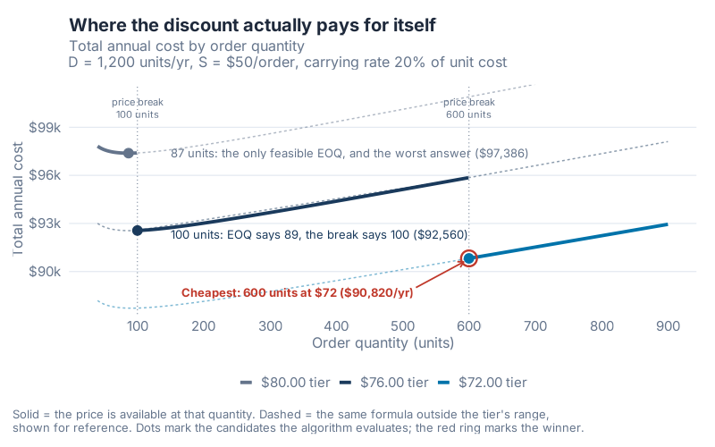
The winner isn’t sitting at the bottom of its own curve, and that’s the part that repays a second look. The $72.00 curve bottoms out at 91 units. If your supplier sold 91 units at $72.00, you’d pay $87,715 a year. Nobody sells that. The cheapest quantity that actually earns the $72.00 price is 600 units, which throws away $3,105 of the discount’s theoretical value and still beats everything reachable by $1,740. The optimum here is knowingly the wrong lot size, parked on the rising limb of its own curve, winning anyway.
The two breaks aren’t the same kind of decision, either. Buying 100 instead of the ideal 89 forfeits about $9 a year, because you’re only eleven units past where the formula wanted to stop. Reaching the second break forfeits $3,105. One is a rounding error. The other is a real commitment that happens to pay.
Now compare 600 units against the naive approach, which is to compute EOQ once at today’s price and order 87 units forever. That costs $97,386 a year. The optimum costs $90,820. You save $6,566 a year, 6.7% of the naive total, on a single part number.
Here’s the honest breakdown, because the headline hides something:
| Component | 87 units @ $80 | 600 units @ $72 | Change |
|---|---|---|---|
| Purchase | $96,000 | $86,400 | −$9,600 |
| Ordering | $693 | $100 | −$593 |
| Holding | $693 | $4,320 | +$3,627 |
| Total | $97,386 | $90,820 | −$6,566 |
Your holding cost goes up more than sixfold. It rises by $3,627 and you still win by $6,566, because the purchase saving is more than two and a half times larger. Any analysis that stops at "big orders tie up cash" would have talked you out of the right answer.
And the right answer has consequences somebody has to live with. Two purchase orders a year instead of twelve. Six months of stock on the floor instead of one. Average inventory value climbing from $3,800 to $21,600, which is $17,800 of additional working capital parked in a rack. Hold that number. It comes back.
Back to That 600th Unit
Now put it in annual terms. 599 units costs $95,853 a year, 600 units costs $90,820. One more unit saves $5,033. If your MRP system is proposing 599 of anything, someone should look at it.
Double the Carrying Rate and the Answer Flips
Everything above rests on i = 20%. That number is an assumption, and it’s usually inherited rather than measured.
So double it. Same quote, same demand, same ordering cost, carrying rate at 40%:
| Candidate | Purchase | Ordering | Holding | Total annual cost |
|---|---|---|---|---|
| 61 units @ $80.00 | $96,000 | $980 | $980 | $97,960 |
| 100 units @ $76.00 | $91,200 | $600 | $1,520 | $93,320 |
| 600 units @ $72.00 | $86,400 | $100 | $8,640 | $95,140 |
The winner changes. At 40%, buying 100 units at $76.00 beats the deep discount by $1,820 a year, 2.0% of the winning total.
The naive answer stays in last place. Computing EOQ at today’s price now gives 61 units at $97,960, which is $4,640 a year worse than the winner, or 4.7% of its own total. Worst at 20%, worst again at 40%. Only the winner’s identity moved.
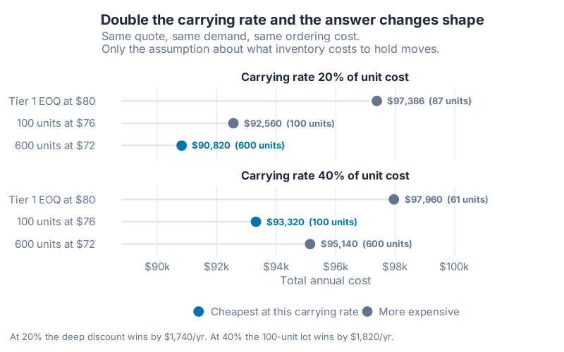
What makes me uncomfortable about this chart is how little had to move. Not the quote. Not demand. Not ordering cost. One assumption I doubt most companies have ever audited, and the recommendation reverses.
Two things deserve a second look. The decision flips completely while the money barely moves: the winning annual cost shifts from $90,820 to $93,320, a gap of 2.8%.
The second one is sharper. On this quote, the textbook move of computing EOQ at today’s price doesn’t just lose at 20% and 40%. It loses everywhere. Buying at tier 1 means paying $96,000 a year for the parts alone, and the 100-unit lot costs less than that in total, including ordering and holding. So the 100-unit lot beats the tier-1 EOQ policy outright at every carrying rate below 110%. That’s arithmetic, not simulation. The guarantee comes from this quote’s first break being deep enough to dominate, so a shallower one wouldn’t hand you the same result.
Notice what both winners have in common. One hundred units is tier 2’s minimum and 600 is tier 3’s minimum, so at any rate below that 110% ceiling, the answer is a price break. Never an interior lot size.
The flip decomposes cleanly: you pay $4,800 more for the parts and $500 more in paperwork in order to dodge $7,120 of carrying cost. Net saving $1,820.
The Discount Is an Investment Offer at 29.8%
Only two candidates are still serious, the 100-unit lot and the 600-unit lot. Find the carrying rate where they tie. Total annual cost is a straight line in the carrying rate once the lot size is fixed, which makes this a crossing point rather than a search.
It lands at 29.8%. At that rate both policies cost $92,931 a year and you should be indifferent.
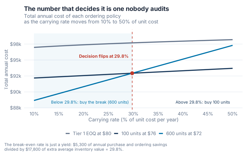
One detail turns this chart into something you can read at a glance. The slope of each line is that policy’s average inventory value. That’s the whole chart. The 100-unit line climbs at $3,800 for every unit of carrying rate, which is 50 units times $76.00. The 600-unit line climbs at $21,600, which is 300 units times $72.00. Those slopes are your working-capital exposure, drawn to scale.
The crossing point isn’t interesting as geometry. Look at what the ratio is made of.
Take everything the bigger lot saves before carrying cost: $4,800 a year on purchase price, plus $500 a year in avoided ordering cost. That’s $5,300. Now take the extra average inventory value it commits, the $17,800 from earlier. Divide.
$5,300 divided by $17,800 is 29.8%.
Your supplier isn’t offering you a discount. They’re offering you a 29.8% annual return on $17,800 of working capital, and asking you to fund it. Take the deal if your real carrying cost is below 29.8%. Refuse it if it’s above. That’s the entire decision, and it’s a treasury decision wearing a procurement costume.
My view is that the break-even rate is the only output of this exercise worth putting in front of a decision-maker. The optimal quantity is an answer. The break-even rate tells you how much your answer can be trusted, which is the more useful thing to know when you’re the one signing.
Notice where 29.8% sits relative to whatever rate your business assumes. Then check your error bars. If your assumed rate could plausibly land on either side of it, you don’t have a decision. You have a coin flip with a spreadsheet attached, and the honest move is to go measure i before you sign anything.
All-Units Versus Incremental, at Real Volume
Part 1 showed that reading the same tier table under incremental rules instead of all-units rules changed a ten-unit order from $690 to $726. Thirty-six dollars. Easy to shrug at.
Put the same question to a part that moves 1,200 units a year and the shrug gets expensive.
Under all-units rules, a 600-unit lot costs $72.00 a unit and $90,820 a year. Under incremental rules, where each tier’s price applies only to the units inside that tier, the same 600-unit lot averages $76.65 a unit and costs $96,683 a year. Identical tier table, identical lot size, $5,863 more, 6.5% worse.
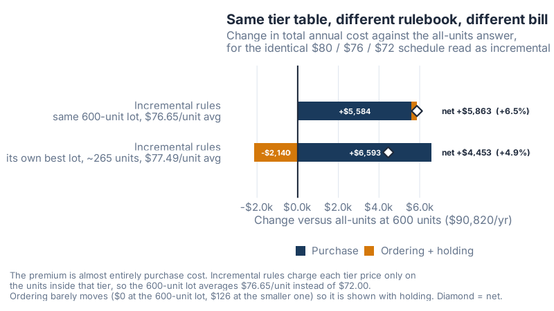
The premium is almost entirely purchase cost. Ordering doesn’t move at 600 units, since both rulebooks place two orders a year. You’re not paying for worse logistics. You’re paying for a different way of counting the same units.
The lower bar caught me out. The two rulebooks don’t even want the same lot size. Under incremental rules the best lot is about 265 units, not 600, and it still costs $95,273 a year, which is $4,453 (4.9%) worse than the all-units optimum.
So re-optimizing helps, and it doesn’t rescue you. Moving to about 265 units saves $1,410 against running incremental rules at 600, then still loses to all-units by $4,453. You can’t out-clever the rulebook.
One caveat on that 265, because precision here would be false. The incremental cost curve is almost flat through that whole neighborhood, varying by roughly five cents across quantities on either side. Treat it as "about 265 units". The real finding is that under incremental rules the lot size barely matters, which tells you the discount has stopped doing any work.
If your quote doesn’t state in writing which rulebook applies, that’s not a formatting oversight. On this part it’s a $5,863 ambiguity.
What This Changes at the Negotiation Table
Plenty of discount schedules in the wild were never designed. They grew. Munson and Rosenblatt (1998) put the theory next to a field study of 39 firms and the two didn’t line up neatly, which is worth knowing before you assume the schedule in front of you was engineered. The models in the literature, from Monahan (1984) to Lal and Staelin (1984), describe schedules built to optimize something.
That asymmetry is your opening. Four asks that work better than "sharpen your pencil":
Move the break, not the price. When your optimum lands on a tier minimum, the breakpoint is doing the damage. On our quote, the 600-unit break forces six months of stock. Ask what a 300-unit break would cost. Sales representatives can often move a threshold when they can’t move a price, because the threshold isn’t in anybody’s margin report.
Quote the break-even rate back to them. "Your 600-unit tier is a 29.8% return on $17,800 of my working capital" reframes the conversation from haggling to underwriting.
Ask which rulebook applies, in writing. All-units or incremental. On this part the difference is $5,863 a year.
Bring the flip. Showing that your answer changes at 29.8% tells the supplier their discount is marginal for you. That’s a stronger position than pretending it’s obviously bad.
Key Takeaways
-
Three numbers turn a price schedule into a decision. Annual demand, ordering cost, and carrying rate. Without them you can audit a supplier’s pricing but you cannot choose an order quantity.
-
The EOQ formula is the least important input. All three tier EOQs here landed between 86 and 92 units, because price only enters under a square root. Breakpoints and carrying rate decide the outcome.
-
The optimum sits at a price break, not at an EOQ. Six hundred units at $72.00 costs $90,820 a year and beats the naive 87-unit answer by $6,566, or 6.7%, on one part number.
-
Holding cost rising is not a reason to say no. The winning policy raises holding cost by $3,627 and still wins by $6,566. Judge the total, never a component.
-
The break-even carrying rate is a yield. $5,300 of annual savings divided by $17,800 of extra inventory value gives 29.8%. Below that, buy the break. Above it, don’t.
-
Doubling the carrying rate reverses the recommendation. At 40% the answer becomes 100 units at $76.00. If your assumed rate is a round number nobody has audited, your inventory policy rests on it anyway.
-
The rulebook is worth 6.5%. The same tier table read as incremental costs $96,683 instead of $90,820 for the identical 600-unit lot.
Your Next Steps
-
Measure your ordering cost this week. Time one buyer through one purchase order end to end, including goods receipt and invoice matching. Multiply by loaded hourly cost. You now have S, and it’s almost certainly not the number in your ERP’s default field.
-
Pull the carrying rate your business actually uses and find out who set it. Cost of capital, storage, insurance, shrinkage, obsolescence. If the answer is "20%, it’s always been 20%", you’ve found the assumption quietly steering every lot-size decision you make.
-
Run the break-even calculation on your three largest tiered parts. Use the
be_rate()function in the R code below. If the break-even rate lands inside the range your carrying rate could plausibly take, stop optimizing and go measure the rate instead. -
Grep your open quotes for the words "all-units" and "incremental". Any quote with tiers and neither word is ambiguous by 6.5% on this example. Send one email per supplier and get it in writing.
-
Check your MRP for order proposals sitting just below a price break. Anything proposing 599 when 600 changes the price is leaving money on the table, and on this part the 600th unit reduces the invoice by $2,324.00.
-
Put the break-even rate, not the optimal quantity, in your next approval request. For what large minimum lots do to working capital, see The Most Expensive Word in Procurement: Minimum. For the base formula, see The $2,700 Post-It Note.
Interactive Dashboard
The Part 1 calculator has been upgraded. It still does the original job. Paste in a tier table, get a one-line verdict on whether the schedule hides a roller-coaster, and read the counter-offer price that fixes it. Share links still work.
New for Part 2: click Annual Cost Example. It loads this post’s scenario and reproduces the candidate table, the optimum, and the break-even rate. Then tick Price-break EOQ and it runs the algorithm on your own quote, marking which tier EOQs are feasible, which collapse to a break, and which lot wins. A sensitivity line underneath names your break-even rate and the winner on each side. Test the 29.8% argument instead of trusting it.
Two limits. The annual-cost analysis is all-units only, because incremental lot sizing is a different algorithm. The All-units and Incremental buttons still compare both rulebooks on your tier table, but the annual incremental figures above come from the R code, not the calculator.
Then do one thing. Change Holding rate i (%/yr) from 20 to 40 and watch the recommendation flip from 600 units to 100. One number, reversed answer.
Interactive Dashboard
Explore the data yourself — adjust parameters and see the results update in real time.
References
- Crowther, J. F. (1964). Rationale for Quantity Discounts. Harvard Business Review, 42 (March–April), 121–127.
- Monahan, J. P. (1984). A Quantity Discount Pricing Model to Increase Vendor Profits. Management Science, 30(6), 720–726. doi.org/10.1287/mnsc.30.6.720
- Lal, R., & Staelin, R. (1984). An Approach for Developing an Optimal Discount Pricing Policy. Management Science, 30(12), 1524–1539. doi.org/10.1287/mnsc.30.12.1524
- Dolan, R. J. (1987). Quantity Discounts: Managerial Issues and Research Opportunities. Marketing Science, 6(1), 1–22. doi.org/10.1287/mksc.6.1.1
- Tersine, R. J., & Barman, S. (1991). Economic Inventory/Transport Lot Sizing with Quantity and Freight Rate Discounts. Decision Sciences, 22(5), 1171–1179. doi.org/10.1111/j.1540-5915.1991.tb01914.x
- Benton, W. C., & Park, S. (1996). A classification of literature on determining the lot size under quantity discounts. European Journal of Operational Research, 92(2), 219–238.
- Munson, C. L., & Rosenblatt, M. J. (1998). Theories and Realities of Quantity Discounts: An Exploratory Study. Production and Operations Management, 7(4), 352–369. doi.org/10.1111/j.1937-5956.1998.tb00129.x
Show R Code
One setup note before you run it. The script opens with source("Scripts/theme_inphronesys.R"), which is this blog’s shared ggplot2 theme. If you don’t have that file, replace that line with theme_minimal(base_size = 13) and everything else runs unchanged. Section 9 at the bottom, "Apply to Your Own Data", is where you swap in your own demand, ordering cost, carrying rate, and tier table.
# =============================================================================
# generate_qda2_images.R
# "Quantity Discount Analysis, Part 2" — price-break EOQ (July 2026)
# -----------------------------------------------------------------------------
# Part 1 asked: is this discount schedule honest? (incremental cost per tier)
# Part 2 asks the harder question: how much should I actually order?
#
# Answering it requires three parameters the quote sheet never mentions:
# annual demand D, ordering cost S, and the carrying rate i (percent of unit
# cost per year). Feed those into the classic price-break EOQ algorithm:
#
#   1. For every tier price p_j, compute the unconstrained EOQ:
#        Q_j* = sqrt(2 * D * S / (i * p_j))
#   2. If Q_j* falls inside tier j's quantity range it is FEASIBLE.
#      If it falls below the tier minimum, the tier can only be reached by
#      buying up to that minimum, so the minimum becomes the candidate.
#      If it falls above the tier maximum, the tier is dominated (drop it).
#   3. Evaluate the total annual cost of every surviving candidate:
#        TAC(Q) = D * p(Q) + (D / Q) * S + (Q / 2) * i * p(Q)
#              = purchase   + ordering    + holding
#   4. The global minimum wins.
#
# Every number in the post comes out of this script. Nothing is hand-typed.
#
# Run from the project root:  Rscript Scripts/generate_qda2_images.R
# =============================================================================

source("Scripts/theme_inphronesys.R")

suppressPackageStartupMessages({
  library(ggplot2)
  library(dplyr)
  library(tidyr)
  library(scales)
})

options(scipen = 999)
img_dir <- "Images"
if (!dir.exists(img_dir)) dir.create(img_dir)

# =============================================================================
# 1. SCENARIO — one machined aluminium housing, three-tier all-units schedule
# =============================================================================

D <- 1200      # annual demand, units
S <- 50        # ordering cost, $ per purchase order
I_BASE <- 0.20 # carrying rate, fraction of unit cost per year
I_HIGH <- 0.40 # stress case: carrying rate doubled

schedule <- data.frame(
  tier    = 1:3,
  qty_min = c(1, 100, 600),
  qty_max = c(99, 599, Inf),
  price   = c(80, 76, 72)
)

# Unit price that actually applies to an order of q units (all-units rules)
price_at <- function(q, sched = schedule) sched$price[findInterval(q, sched$qty_min)]

# Total annual cost, all-units rules
tac_all_units <- function(q, price, i) D * price + (D / q) * S + (q / 2) * i * price

# Unconstrained EOQ at a given unit price
eoq_at <- function(price, i) sqrt(2 * D * S / (i * price))

# =============================================================================
# 2. THE PRICE-BREAK EOQ ALGORITHM
# =============================================================================

price_break_eoq <- function(sched, i) {
  cand <- lapply(seq_len(nrow(sched)), function(k) {
    q_uncon <- eoq_at(sched$price[k], i)
    status <- if (q_uncon < sched$qty_min[k]) {
      "below tier minimum"
    } else if (q_uncon > sched$qty_max[k]) {
      "above tier maximum"
    } else {
      "feasible"
    }
    # A tier whose EOQ sits below its minimum is still reachable: buy up to
    # the break. A tier whose EOQ sits above its maximum is dominated by the
    # next tier down and drops out.
    q_eval <- switch(status,
      "feasible"           = q_uncon,
      "below tier minimum" = sched$qty_min[k],
      "above tier maximum" = NA_real_
    )
    data.frame(
      tier         = sched$tier[k],
      price        = sched$price[k],
      eoq_uncon    = q_uncon,
      status       = status,
      q_eval       = q_eval,
      candidate    = ifelse(status == "feasible", "feasible EOQ", "tier minimum"),
      stringsAsFactors = FALSE
    )
  })
  out <- do.call(rbind, cand)
  out <- out[!is.na(out$q_eval), ]
  out$purchase <- D * out$price
  out$ordering <- (D / out$q_eval) * S
  out$holding  <- (out$q_eval / 2) * i * out$price
  out$tac      <- out$purchase + out$ordering + out$holding
  out$is_best   <- out$tac == min(out$tac)
  out[order(out$q_eval), ]
}

cand_base <- price_break_eoq(schedule, I_BASE)
cand_high <- price_break_eoq(schedule, I_HIGH)

cat("\n================ CANDIDATES AT i = 20% ================\n")
print(cand_base, digits = 8, row.names = FALSE)
cat("\n================ CANDIDATES AT i = 40% ================\n")
print(cand_high, digits = 8, row.names = FALSE)

best_base <- cand_base[cand_base$is_best, ]
best_high <- cand_high[cand_high$is_best, ]
cat(sprintf("\nOptimal at 20%%: %.4f units @ $%.2f, TAC = %.4f\n",
            best_base$q_eval, best_base$price, best_base$tac))
cat(sprintf("Optimal at 40%%: %.4f units @ $%.2f, TAC = %.4f\n",
            best_high$q_eval, best_high$price, best_high$tac))

# --- The break-even carrying rate between the two serious candidates --------
# TAC(Q) is linear in i:  TAC(Q) = [D*p + (D/Q)*S] + [(Q/2)*p] * i
# Set the two lines equal and solve for i.
be_rate <- function(q_a, p_a, q_b, p_b) {
  int_a <- D * p_a + (D / q_a) * S; slope_a <- (q_a / 2) * p_a
  int_b <- D * p_b + (D / q_b) * S; slope_b <- (q_b / 2) * p_b
  (int_a - int_b) / (slope_b - slope_a)
}
i_star <- be_rate(100, 76, 600, 72)
cat(sprintf("\nBreak-even carrying rate between Q=100 and Q=600: %.6f (%.2f%%)\n",
            i_star, i_star * 100))
cat(sprintf("  savings before carrying cost = purchase %.2f + ordering %.2f = %.2f\n",
            D * (76 - 72), (D / 100) * S - (D / 600) * S, D * (76 - 72) + (D / 100) * S - (D / 600) * S))
cat(sprintf("  extra average inventory value = %.2f - %.2f = %.2f\n",
            (600 / 2) * 72, (100 / 2) * 76, (600 / 2) * 72 - (100 / 2) * 76))
cat(sprintf("  ratio = %.2f / %.2f = %.6f\n",
            D * (76 - 72) + (D / 100) * S - (D / 600) * S,
            (600 / 2) * 72 - (100 / 2) * 76, i_star))

# =============================================================================
# 3. INCREMENTAL DISCOUNT RULES ON THE SAME TIER TABLE
# =============================================================================
# Under incremental rules each tier's price applies only to the units inside
# that tier, so the order's acquisition cost is a piecewise sum and the
# average unit cost depends on Q. Holding cost is valued at that average
# acquisition cost (standard treatment): holding = i * C(Q) / 2.

units_in_tier <- function(q, sched = schedule) {
  pmax(0, pmin(q, sched$qty_max) - sched$qty_min + 1)
}
acq_cost_incremental <- function(q, sched = schedule) sum(units_in_tier(q, sched) * sched$price)

tac_incremental <- function(q, i, sched = schedule) {
  ct <- acq_cost_incremental(q, sched)
  D * (ct / q) + (D / q) * S + i * ct / 2
}

q_opt <- best_base$q_eval                       # 600 under all-units rules
c_incr_at_opt <- acq_cost_incremental(q_opt)
avg_price_incr <- c_incr_at_opt / q_opt

grid_q <- 1:3000
tac_incr_grid <- vapply(grid_q, tac_incremental, numeric(1), i = I_BASE)
q_opt_incr <- grid_q[which.min(tac_incr_grid)]

cat("\n================ INCREMENTAL RULES (i = 20%) ================\n")
cat(sprintf("units per tier at Q = %g: %s\n", q_opt,
            paste(units_in_tier(q_opt), collapse = " / ")))
cat(sprintf("C(%g) = %.2f  ->  average unit cost = %.6f\n", q_opt, c_incr_at_opt, avg_price_incr))
cat(sprintf("TAC incremental at Q = %g: %.4f  (all-units: %.4f, gap %.4f = %.4f%%)\n",
            q_opt, tac_incremental(q_opt, I_BASE), best_base$tac,
            tac_incremental(q_opt, I_BASE) - best_base$tac,
            (tac_incremental(q_opt, I_BASE) - best_base$tac) / best_base$tac * 100))
cat(sprintf("Incremental rules own optimum: Q = %d, TAC = %.4f (gap vs all-units optimum %.4f)\n",
            q_opt_incr, min(tac_incr_grid), min(tac_incr_grid) - best_base$tac))

# Part 1 continuity: the incremental cost of the 600th unit under all-units rules
cat(sprintf("\nAll-units purchase cost at 599 units: %.2f ; at 600 units: %.2f ; the 600th unit moves it by %.2f\n",
            599 * 76, 600 * 72, 600 * 72 - 599 * 76))
cat(sprintf("TAC at 599 units: %.4f ; at 600 units: %.4f ; one more unit saves %.4f\n",
            tac_all_units(599, 76, I_BASE), best_base$tac,
            tac_all_units(599, 76, I_BASE) - best_base$tac))

# =============================================================================
# 4. CHART 1 — the algorithm on one page
# =============================================================================

curve_df <- expand.grid(qty = seq(40, 900, by = 1), tier = 1:3) %>%
  mutate(
    price     = schedule$price[tier],
    tac       = tac_all_units(qty, price, I_BASE),
    feasible  = qty >= schedule$qty_min[tier] & qty <= schedule$qty_max[tier],
    price_lab = factor(paste0("$", format(price, nsmall = 2), " tier"),
                       levels = c("$80.00 tier", "$76.00 tier", "$72.00 tier"))
  )

tier_cols <- c("$80.00 tier" = iph_colors$grey,
               "$76.00 tier" = iph_colors$navy,
               "$72.00 tier" = iph_colors$blue)

pts <- cand_base %>%
  mutate(price_lab = factor(paste0("$", format(price, nsmall = 2), " tier"),
                            levels = levels(curve_df$price_lab)))

p1 <- ggplot(curve_df, aes(x = qty, y = tac, colour = price_lab)) +
  geom_line(data = filter(curve_df, !feasible),
            aes(group = price_lab), linewidth = 0.5, linetype = "22", alpha = 0.5) +
  geom_line(data = filter(curve_df, feasible),
            aes(group = price_lab), linewidth = 1.3) +
  geom_vline(xintercept = c(100, 600), linewidth = 0.35,
             linetype = "dotted", colour = iph_colors$grey) +
  geom_point(data = pts, aes(x = q_eval, y = tac), size = 3.2, show.legend = FALSE) +
  geom_point(data = filter(pts, is_best), aes(x = q_eval, y = tac),
             size = 5.2, shape = 21, stroke = 1.2, fill = NA,
             colour = iph_colors$red, show.legend = FALSE) +
  annotate("text", x = 100, y = 100200, label = "price break\n100 units",
           size = 3, colour = iph_colors$grey, lineheight = 0.95) +
  annotate("text", x = 600, y = 100200, label = "price break\n600 units",
           size = 3, colour = iph_colors$grey, lineheight = 0.95) +
  annotate("text", x = 150, y = 97386, hjust = 0, size = 3.3, colour = iph_colors$grey,
           label = "87 units: the only feasible EOQ, and the worst answer ($97,386)") +
  annotate("text", x = 150, y = 92300, hjust = 0, size = 3.3, colour = iph_colors$navy,
           label = "100 units: EOQ says 89, the break says 100 ($92,560)") +
  annotate("segment", x = 520, xend = 592, y = 89000, yend = 90600,
           colour = iph_colors$red, linewidth = 0.6,
           arrow = arrow(length = unit(0.18, "cm"))) +
  annotate("text", x = 515, y = 88700, hjust = 1, size = 3.5, fontface = "bold",
           colour = iph_colors$red, label = "Cheapest: 600 units at $72 ($90,820/yr)") +
  scale_colour_manual(values = tier_cols) +
  scale_x_continuous(breaks = c(100, 200, 300, 400, 500, 600, 700, 800, 900),
                     labels = comma_format()) +
  scale_y_continuous(labels = dollar_format(scale = 0.001, suffix = "k", accuracy = 1)) +
  coord_cartesian(xlim = c(40, 900), ylim = c(88000, 101000)) +
  labs(
    title = "Where the discount actually pays for itself",
    subtitle = paste0("Total annual cost by order quantity\n",
                      "D = 1,200 units/yr, S = $50/order, carrying rate 20% of unit cost"),
    x = "Order quantity (units)",
    y = "Total annual cost",
    colour = NULL,
    caption = paste0("Solid = the price is available at that quantity. ",
                     "Dashed = the same formula outside the tier's range,\n",
                     "shown for reference. Dots mark the candidates the algorithm evaluates; ",
                     "the red ring marks the winner.")
  ) +
  theme_inphronesys(grid = "y") +
  theme(plot.caption.position = "plot")

ggsave(file.path(img_dir, "qda2_total_cost_curves.png"), p1,
       width = 8, height = 5, dpi = 100, bg = "white")
cat("\nsaved: qda2_total_cost_curves.png\n")

# =============================================================================
# 5. CHART 2 — the carrying-rate flip
# =============================================================================

policy_levels <- c("600 units at $72", "100 units at $76", "Tier 1 EOQ at $80")

flip_df <- bind_rows(
  cand_base %>% mutate(rate = "Carrying rate 20% of unit cost"),
  cand_high %>% mutate(rate = "Carrying rate 40% of unit cost")
) %>%
  mutate(
    policy = case_when(
      price == 72 ~ "600 units at $72",
      price == 76 ~ "100 units at $76",
      TRUE        ~ "Tier 1 EOQ at $80"
    ),
    policy = factor(policy, levels = policy_levels),
    rate   = factor(rate, levels = c("Carrying rate 20% of unit cost",
                                     "Carrying rate 40% of unit cost")),
    verdict = ifelse(is_best, "Cheapest at this carrying rate", "More expensive"),
    lab = paste0(dollar(tac, accuracy = 1), "  (", comma(round(q_eval)), " units)")
  )

p2 <- ggplot(flip_df, aes(x = tac, y = policy, colour = verdict)) +
  geom_segment(aes(x = 88800, xend = tac, yend = policy),
               colour = iph_colors$lightgrey, linewidth = 0.9) +
  geom_point(size = 4.2) +
  geom_text(aes(label = lab), hjust = 0, nudge_x = 350, size = 3.3,
            fontface = "bold", show.legend = FALSE) +
  facet_wrap(~rate, ncol = 1) +
  scale_colour_manual(values = c("Cheapest at this carrying rate" = iph_colors$blue,
                                 "More expensive" = iph_colors$grey)) +
  scale_x_continuous(labels = dollar_format(scale = 0.001, suffix = "k", accuracy = 1),
                     breaks = seq(90000, 100000, by = 2000)) +
  coord_cartesian(xlim = c(88800, 102500)) +
  labs(
    title = "Double the carrying rate and the answer changes shape",
    subtitle = paste0("Same quote, same demand, same ordering cost.\n",
                      "Only the assumption about what inventory costs to hold moves."),
    x = "Total annual cost", y = NULL, colour = NULL,
    caption = "At 20% the deep discount wins by $1,740/yr. At 40% the 100-unit lot wins by $1,820/yr."
  ) +
  theme_inphronesys(grid = "x") +
  theme(legend.position = "bottom", plot.caption.position = "plot")

ggsave(file.path(img_dir, "qda2_holding_rate_flip.png"), p2,
       width = 8, height = 5, dpi = 100, bg = "white")
cat("saved: qda2_holding_rate_flip.png\n")

# =============================================================================
# 6. CHART 3 — the break-even carrying rate
# =============================================================================

rate_grid <- seq(0.10, 0.50, by = 0.0025)
be_df <- bind_rows(
  data.frame(i = rate_grid,
             policy = "Tier 1 EOQ at $80",
             tac = vapply(rate_grid, function(i) tac_all_units(eoq_at(80, i), 80, i), numeric(1))),
  data.frame(i = rate_grid, policy = "100 units at $76",
             tac = tac_all_units(100, 76, rate_grid)),
  data.frame(i = rate_grid, policy = "600 units at $72",
             tac = tac_all_units(600, 72, rate_grid))
) %>%
  mutate(policy = factor(policy, levels = c("Tier 1 EOQ at $80",
                                            "100 units at $76",
                                            "600 units at $72")))

tac_at_star <- tac_all_units(600, 72, i_star)

p3 <- ggplot(be_df, aes(x = i, y = tac, colour = policy)) +
  annotate("rect", xmin = 0.10, xmax = i_star, ymin = 87500, ymax = 99200,
           fill = iph_colors$blue, alpha = 0.05) +
  geom_vline(xintercept = i_star, linetype = "dashed",
             colour = iph_colors$red, linewidth = 0.6) +
  geom_line(linewidth = 1.2) +
  annotate("point", x = i_star, y = tac_at_star, colour = iph_colors$red, size = 3.4) +
  annotate("text", x = i_star - 0.008, y = 95600, hjust = 1, size = 3.6, fontface = "bold",
           colour = iph_colors$red, label = "Decision flips at 29.8%") +
  annotate("text", x = 0.135, y = 88400, hjust = 0, size = 3.4, colour = iph_colors$blue,
           label = "Below 29.8%: buy the break (600 units)") +
  annotate("text", x = 0.495, y = 88400, hjust = 1, size = 3.4, colour = iph_colors$navy,
           label = "Above 29.8%: buy 100 units") +
  scale_colour_manual(values = c("Tier 1 EOQ at $80" = iph_colors$grey,
                                 "100 units at $76" = iph_colors$navy,
                                 "600 units at $72" = iph_colors$blue)) +
  scale_x_continuous(labels = percent_format(accuracy = 1),
                     breaks = seq(0.10, 0.50, by = 0.05)) +
  scale_y_continuous(labels = dollar_format(scale = 0.001, suffix = "k", accuracy = 1)) +
  coord_cartesian(ylim = c(87800, 99200)) +
  labs(
    title = "The number that decides it is one nobody audits",
    subtitle = paste0("Total annual cost of each ordering policy\n",
                      "as the carrying rate moves from 10% to 50% of unit cost"),
    x = "Carrying rate (% of unit cost per year)",
    y = "Total annual cost",
    colour = NULL,
    caption = paste0("The break-even rate is just a yield: $5,300 of annual purchase and ordering ",
                     "savings\ndivided by $17,800 of extra average inventory value = 29.8%.")
  ) +
  theme_inphronesys(grid = "y") +
  theme(plot.caption.position = "plot")

ggsave(file.path(img_dir, "qda2_breakeven_holding_rate.png"), p3,
       width = 8, height = 5, dpi = 100, bg = "white")
cat("saved: qda2_breakeven_holding_rate.png\n")

# =============================================================================
# 7. CHART 4 — all-units vs incremental rules on the identical tier table
# =============================================================================

# Plotted as CHANGE against the all-units optimum rather than as three near-equal
# absolute totals. Absolute stacked bars put 90,820 / 96,683 / 95,273 within 6% of
# each other, which renders the whole argument invisible and leaves the text labels
# doing the work the marks should do. Differencing makes zero a real reference point
# (the all-units answer), so a zero-based axis is honest here rather than misleading,
# and it also exposes WHY the rulebook costs more: the premium is purchase cost.

incr_opt_c <- acq_cost_incremental(q_opt_incr)

comp_all_units <- c(purchase = D * 72,
                    ordering = (D / 600) * S,
                    holding  = (600 / 2) * I_BASE * 72)
comp_incr_600  <- c(purchase = D * avg_price_incr,
                    ordering = (D / 600) * S,
                    holding  = I_BASE * c_incr_at_opt / 2)
comp_incr_opt  <- c(purchase = D * (incr_opt_c / q_opt_incr),
                    ordering = (D / q_opt_incr) * S,
                    holding  = I_BASE * incr_opt_c / 2)

# Ordering changes by $0 at the 600-unit lot and $126 at the smaller one, which is
# sub-pixel against a 14k axis. Shown as its own fill it would advertise a legend
# colour the reader cannot find, so it is combined with holding. The two segments
# then sum exactly to the net, which a dropped component would not.
make_delta_row <- function(label, comp) {
  d <- comp - comp_all_units
  data.frame(label = label,
             component = c("Purchase", "Ordering + holding"),
             value = c(as.numeric(d["purchase"]),
                       as.numeric(d["ordering"] + d["holding"])),
             stringsAsFactors = FALSE)
}

delta_df <- bind_rows(
  make_delta_row(paste0("Incremental rules\nsame 600-unit lot, $",
                        format(round(avg_price_incr, 2), nsmall = 2), "/unit avg"), comp_incr_600),
  make_delta_row(paste0("Incremental rules\nits own best lot, ~", q_opt_incr, " units, $",
                        format(round(incr_opt_c / q_opt_incr, 2), nsmall = 2), "/unit avg"),
                 comp_incr_opt)
) %>%
  mutate(
    label = factor(label, levels = rev(unique(label))),
    component = factor(component, levels = c("Purchase", "Ordering + holding"))
  )

net_df <- delta_df %>%
  group_by(label) %>%
  summarise(net = sum(value), .groups = "drop") %>%
  mutate(lab = paste0("net +", dollar(net, accuracy = 1),
                      "  (+", percent(net / best_base$tac, accuracy = 0.1), ")"))

cat("\ncomponent changes versus all-units at 600 units (chart 4):\n")
print(delta_df, row.names = FALSE, digits = 8)
print(net_df, row.names = FALSE, digits = 8)

p4 <- ggplot(delta_df, aes(x = value, y = label, fill = component)) +
  geom_col(width = 0.45, position = position_stack(reverse = TRUE)) +
  geom_vline(xintercept = 0, colour = iph_colors$dark, linewidth = 0.7) +
  # Net change marker, so a bar with a negative segment cannot be misread as its total
  geom_point(data = net_df, aes(x = net, y = label), inherit.aes = FALSE,
             shape = 23, size = 3.4, fill = "white", stroke = 1.1,
             colour = iph_colors$dark) +
  # Net label sits in a fixed right-hand column, clear of every segment label
  geom_text(data = net_df, aes(x = 7100, y = label, label = lab), inherit.aes = FALSE,
            hjust = 0, size = 3.2, fontface = "bold", colour = iph_colors$dark) +
  # Label only the segments wide enough to hold text
  geom_text(data = filter(delta_df, abs(value) >= 1000),
            aes(label = dollar(value, accuracy = 1, style_positive = "plus")),
            position = position_stack(reverse = TRUE, vjust = 0.5),
            size = 3, colour = "white", fontface = "bold", show.legend = FALSE) +
  scale_fill_manual(values = c("Purchase" = iph_colors$navy,
                               "Ordering + holding" = iph_colors$orange)) +
  scale_x_continuous(labels = dollar_format(scale = 0.001, suffix = "k", accuracy = 0.1),
                     breaks = seq(-2000, 6000, by = 2000)) +
  coord_cartesian(xlim = c(-2800, 11200), ylim = c(0.5, 2.5)) +
  labs(
    title = "Same tier table, different rulebook, different bill",
    subtitle = paste0("Change in total annual cost against the all-units answer,\n",
                      "for the identical $80 / $76 / $72 schedule read as incremental discounts"),
    x = "Change versus all-units at 600 units ($90,820/yr)",
    y = NULL, fill = NULL,
    caption = paste0("The premium is almost entirely purchase cost. Incremental rules charge each tier ",
                     "price only on\nthe units inside that tier, so the 600-unit lot averages ",
                     "$76.65/unit instead of $72.00.\nOrdering barely moves ($0 at the 600-unit lot, ",
                     "$126 at the smaller one) so it is shown with holding. Diamond = net.")
  ) +
  theme_inphronesys(grid = "x") +
  theme(plot.caption.position = "plot")

ggsave(file.path(img_dir, "qda2_allunits_vs_incremental.png"), p4,
       width = 8, height = 4.5, dpi = 100, bg = "white")
cat("saved: qda2_allunits_vs_incremental.png\n")

# =============================================================================
# 8. SUMMARY BLOCK — every number the post is allowed to quote
# =============================================================================

cat("\n==================================================================\n")
cat("QDA PART 2 — FINAL NUMBERS\n")
cat("==================================================================\n")
cat(sprintf("D = %g units/yr, S = $%g/order, tiers: 1-99 @ $80, 100-599 @ $76, 600+ @ $72\n", D, S))

for (nm in c("20%", "40%")) {
  tbl <- if (nm == "20%") cand_base else cand_high
  i <- if (nm == "20%") I_BASE else I_HIGH
  cat(sprintf("\n--- carrying rate %s ---\n", nm))
  for (k in seq_len(nrow(tbl))) {
    r <- tbl[k, ]
    cat(sprintf("  Q = %8.4f @ $%.2f (%s) : purchase %10.4f + ordering %8.4f + holding %9.4f = %11.4f%s\n",
                r$q_eval, r$price, r$candidate, r$purchase, r$ordering, r$holding, r$tac,
                ifelse(r$is_best, "  <== OPTIMAL", "")))
  }
  cat(sprintf("  runner-up gap: %.4f\n", sort(tbl$tac)[2] - min(tbl$tac)))
  cat(sprintf("  unconstrained EOQs: %s\n",
              paste(sprintf("$%.0f -> %.4f (%s)", schedule$price,
                            eoq_at(schedule$price, i),
                            ifelse(eoq_at(schedule$price, i) >= schedule$qty_min &
                                     eoq_at(schedule$price, i) <= schedule$qty_max,
                                   "feasible", "infeasible")), collapse = "; ")))
}

cat(sprintf("\nSavings of the optimum over the naive tier-1 EOQ at 20%%: %.4f (%.4f%% of %.4f)\n",
            cand_base$tac[cand_base$candidate == "feasible EOQ"] - best_base$tac,
            (cand_base$tac[cand_base$candidate == "feasible EOQ"] - best_base$tac) /
              cand_base$tac[cand_base$candidate == "feasible EOQ"] * 100,
            cand_base$tac[cand_base$candidate == "feasible EOQ"]))
cat(sprintf("Break-even carrying rate: %.6f\n", i_star))
cat(sprintf("Orders per year: %.4f (87 units), %.4f (100 units), %.4f (600 units)\n",
            D / eoq_at(80, I_BASE), D / 100, D / 600))
cat(sprintf("Months of supply: %.4f (100 units), %.4f (600 units)\n", 100 / D * 12, 600 / D * 12))
cat(sprintf("Average inventory value: $%.2f at 600 units, $%.2f at 100 units, delta $%.2f\n",
            (600 / 2) * 72, (100 / 2) * 76, (600 / 2) * 72 - (100 / 2) * 76))

# =============================================================================
# 8b. DERIVED FIGURES QUOTED IN THE POST
# =============================================================================
# Anything the post states that is not already a candidate TAC above is derived
# here, so the claim at the top of this file ("every number in the post comes
# out of this script") is literally true and checkable in one place.

cat("\n================ DERIVED FIGURES QUOTED IN THE POST ================\n")

# --- Price steps in the quote -----------------------------------------------
cat(sprintf("price step, list to deepest: %.2f - %.2f = %.2f  (%.2f / %.2f = %.6f)\n",
            80, 72, 80 - 72, 80 - 72, 80, (80 - 72) / 80))
cat(sprintf("price step, tier 2 to tier 3: %.2f - %.2f = %.2f  (%.2f / %.2f = %.6f)\n",
            76, 72, 76 - 72, 76 - 72, 76, (76 - 72) / 76))

# --- Component decomposition, naive EOQ -> optimum at i = 20% ---------------
naive_base <- cand_base[cand_base$candidate == "feasible EOQ", ]
cat(sprintf("\ndecomposition %.4f units -> %.0f units at i = 20%%:\n",
            naive_base$q_eval, best_base$q_eval))
cat(sprintf("  purchase %.4f -> %.4f  = %+.4f\n",
            naive_base$purchase, best_base$purchase, best_base$purchase - naive_base$purchase))
cat(sprintf("  ordering %.4f -> %.4f  = %+.4f\n",
            naive_base$ordering, best_base$ordering, best_base$ordering - naive_base$ordering))
cat(sprintf("  holding  %.4f -> %.4f  = %+.4f\n",
            naive_base$holding, best_base$holding, best_base$holding - naive_base$holding))
cat(sprintf("  net      %.4f -> %.4f  = %+.4f\n",
            naive_base$tac, best_base$tac, best_base$tac - naive_base$tac))

# --- Component decomposition of the flip, 600 -> 100 at i = 40% -------------
flip_from <- cand_high[cand_high$q_eval == 600, ]
flip_to   <- cand_high[cand_high$q_eval == 100, ]
cat("\ndecomposition 600 units -> 100 units at i = 40%:\n")
cat(sprintf("  purchase %.4f -> %.4f  = %+.4f\n",
            flip_from$purchase, flip_to$purchase, flip_to$purchase - flip_from$purchase))
cat(sprintf("  ordering %.4f -> %.4f  = %+.4f\n",
            flip_from$ordering, flip_to$ordering, flip_to$ordering - flip_from$ordering))
cat(sprintf("  holding  %.4f -> %.4f  = %+.4f\n",
            flip_from$holding, flip_to$holding, flip_to$holding - flip_from$holding))
cat(sprintf("  net      %.4f -> %.4f  = %+.4f\n",
            flip_from$tac, flip_to$tac, flip_to$tac - flip_from$tac))

# --- Saving of the optimum over the naive EOQ, both rates -------------------
naive_high <- cand_high[cand_high$candidate == "feasible EOQ", ]
for (nm in c("20%", "40%")) {
  nv <- if (nm == "20%") naive_base else naive_high
  bs <- if (nm == "20%") best_base else best_high
  cat(sprintf("\nsaving vs naive EOQ at i = %s: %.4f - %.4f = %.4f  (%.4f / %.4f = %.6f)\n",
              nm, nv$tac, bs$tac, nv$tac - bs$tac, nv$tac - bs$tac, nv$tac, (nv$tac - bs$tac) / nv$tac))
}

# --- The counterfactual floor of each tier ----------------------------------
# TAC if the tier's own unconstrained EOQ were actually purchasable. This is
# NOT a candidate (the algorithm discards it); it exists only to quantify how
# much of a discount's theoretical value the break quantity forfeits.
cat("\ncounterfactual: TAC at each tier's own EOQ, if the tier had no minimum (i = 20%)\n")
for (k in seq_len(nrow(schedule))) {
  p_k <- schedule$price[k]; q_k <- eoq_at(p_k, I_BASE)
  cat(sprintf("  $%.2f tier: EOQ %.4f -> TAC = %.4f * %.0f + sqrt(2*%g*%g*%.2f*%.2f) = %.4f%s\n",
              p_k, q_k, D, p_k, D, S, I_BASE, p_k, tac_all_units(q_k, p_k, I_BASE),
              ifelse(q_k < schedule$qty_min[k], "  (not purchasable)", "")))
}
floor_deep <- tac_all_units(eoq_at(72, I_BASE), 72, I_BASE)
cat(sprintf("  value forfeited by buying the 600 break instead: %.4f - %.4f = %.4f\n",
            best_base$tac, floor_deep, best_base$tac - floor_deep))

# --- Cost of both policies at the break-even carrying rate -----------------
cat(sprintf("\nat the break-even rate i* = %.7f both policies cost: Q=100 -> %.4f ; Q=600 -> %.4f\n",
            i_star, tac_all_units(100, 76, i_star), tac_all_units(600, 72, i_star)))

# --- Winning-TAC spread across the flip ------------------------------------
cat(sprintf("winning TAC spread across the flip: (%.4f - %.4f) / %.4f = %.6f\n",
            best_high$tac, best_base$tac, best_base$tac,
            (best_high$tac - best_base$tac) / best_base$tac))

# --- Incremental re-optimisation saving ------------------------------------
cat(sprintf("\nincremental rules, re-optimising 600 -> %d units saves: %.4f - %.4f = %.4f\n",
            q_opt_incr, tac_incremental(q_opt, I_BASE), min(tac_incr_grid),
            tac_incremental(q_opt, I_BASE) - min(tac_incr_grid)))
cat(sprintf("...and still loses to all-units at 600 by: %.4f - %.4f = %.4f  (%.4f / %.4f = %.6f)\n",
            min(tac_incr_grid), best_base$tac, min(tac_incr_grid) - best_base$tac,
            min(tac_incr_grid) - best_base$tac, best_base$tac,
            (min(tac_incr_grid) - best_base$tac) / best_base$tac))

# --- Why the tier-1 EOQ policy can never win (analytic bound) --------------
# TAC_EOQ(i) >= D * 80 for every i > 0, since ordering and holding are > 0.
# TAC(100, i) = intercept + slope * i, which stays below D * 80 while
#   i < (D*80 - intercept) / slope.
int_100 <- D * 76 + (D / 100) * S
slp_100 <- (100 / 2) * 76
cat(sprintf("\ntier-1 EOQ policy floor = D * 80 = %.4f\n", D * 80))
cat(sprintf("TAC(100, i) = %.4f + %.4f i, which stays below that floor while\n", int_100, slp_100))
cat(sprintf("  i < (%.4f - %.4f) / %.4f = %.4f / %.4f = %.6f\n",
            D * 80, int_100, slp_100, D * 80 - int_100, slp_100, (D * 80 - int_100) / slp_100))
cat("  => the 100-unit lot strictly beats the tier-1 EOQ policy at every carrying rate below that.\n")

# =============================================================================
# 9. APPLY TO YOUR OWN DATA
# =============================================================================
#
# 1. Replace the four inputs. D and S come from your ERP: D is 12 months of
#    issues for the part, S is the fully loaded cost of raising one purchase
#    order (buyer time + goods receipt + invoice matching, not the whole
#    purchasing department's budget divided by order count). i is the annual
#    carrying rate as a fraction of unit cost: cost of capital + storage +
#    insurance + shrinkage + obsolescence risk. Most companies have never
#    measured their real carrying rate.
#
#      D <- 4800
#      S <- 85
#      I_BASE <- 0.25
#
# 2. Replace the tier table with the supplier's quote. qty_max of the top
#    tier stays Inf. Prices must be the all-units prices from the quote.
#
#      schedule <- data.frame(
#        tier    = 1:4,
#        qty_min = c(1, 250, 1000, 2500),
#        qty_max = c(249, 999, 2499, Inf),
#        price   = c(12.50, 11.80, 11.20, 10.95)
#      )
#
# 3. Run the algorithm and read the table:
#
#      price_break_eoq(schedule, I_BASE)
#
# 4. Find the carrying rate at which your decision flips. If that number is
#    inside the range your own carrying rate could plausibly take, the
#    discount is not a decision, it is a coin flip, and the honest move is to
#    go measure i before signing.
#
#      be_rate(q_a = 250, p_a = 11.80, q_b = 1000, p_b = 11.20)
#
# 5. Check what the same table would cost under incremental rules. If the
#    quote does not say "all-units" or "incremental" in writing, ask. The
#    gap is real money.
#
#      tac_incremental(1000, I_BASE)
#
# =============================================================================

cat("\nAll 4 QDA Part 2 charts generated.\n")
Leave a Reply