Here is a quietly remarkable fact about the forecasting engine buried inside your ERP.
The core algorithm — the one that smooths your demand history, pulls out a trend, teases apart the seasonal swings, and projects the whole thing forward twelve months — was written for the United States Navy. It was written in 1957. It was written on a contract from the Office of Naval Research, at the Carnegie Institute of Technology, by a young operations researcher named Charles C. Holt, whose job was to keep Navy warehouses from running out of parts. The follow-up paper, which added the seasonal component, was written three years later by Holt’s student Peter Winters. Together they produced three recursive formulas, a page of arithmetic, and no calculus beyond a weighted average.
Nearly seven decades later, every commercial forecasting package on Earth still implements those formulas. Excel has them. SAP has them. Oracle has them. The ETS() function in R has them. The sophisticated-looking „demand sensing“ product your CFO just bought for six figures has them, wrapped in a friendlier dashboard. The three equations have been re-derived, extended, and automated into model-selection routines — but at the core, the recursion Holt scratched onto ONR Memorandum 52 is still doing most of the work.
This is the post where we take that method apart — without the formulas. By the end, you will know what α, β, and γ actually do, why Gardner and McKenzie damped the trend in 1985 (and why you should almost always use their version), how the modern ETS framework makes model selection automatic, and — most importantly — which situations Holt-Winters is genuinely the right tool for, versus which situations will make it embarrass you in front of the S&OP committee.
We start where forecasting itself started: in 1956, with a man who looked at a warehouse full of Navy spare parts and decided there had to be a better way than averaging the last twelve months.
A Very Short History of the Smoothing Idea
Robert Brown and the Navy’s Inventory Problem (1956)
In the early 1950s, Robert G. Brown was working as an operations research consultant on a problem that had plagued military logistics since the invention of the warehouse: how do you forecast demand for tens of thousands of different spare parts, most of which move infrequently, using only pencil, paper, and the punched-card machines of the day?
Brown’s answer was deceptively simple. Take your current forecast. Compare it to what actually happened. Update the forecast by a small fraction of the error, and throw the rest away. Call it simple exponential smoothing.
The insight sounds obvious now, but it was revolutionary because it was computable. A clerk with a log table could maintain forecasts for ten thousand parts in an afternoon. The Navy needed that. So did General Electric, and U.S. Steel, and everyone else Brown consulted for over the next decade. Simple exponential smoothing became the de facto standard for inventory forecasting before most companies even had computers.
But it had a problem.
Charles Holt and the Trend Equation (1957)
Simple smoothing assumes the level hovers around some roughly constant value. It has no memory of direction. If your demand has been climbing steadily for three years, simple smoothing does not project it upward — it just sits there, flat, underestimating every future month until the system eventually catches up through sheer inertia.
Charles C. Holt, also working under an Office of Naval Research contract — this time at Carnegie Tech — published the fix in 1957 in ONR Memorandum No. 52. It was a technical report, mimeographed and meant for Navy inventory planners, not academic statisticians. For nearly fifty years it circulated as a working paper before finally being formally published in the International Journal of Forecasting in 2004.
Holt’s insight: if the level is drifting, give it a second equation that tracks how fast it is drifting. Smooth the level as Brown did, but also keep a running estimate of the recent slope. Now the forecast becomes level plus slope projected forward. This is Holt’s linear method.
Holt’s 1957 memo actually went further — it also sketched out a third equation for seasonality. But ONR was paying for inventory forecasting, not journal articles, so Holt moved on. The seasonal extension sat in his memo, largely unread, for three years.
The credibility angle for supply chain readers cannot be overstated: Holt-Winters was not invented by academics for academics. It was invented on a defense contract to solve exactly the problem you are solving today — too many SKUs, too little data per SKU, and a boss who wants a forecast by Friday. The method’s DNA is operational, not theoretical.
Peter Winters and the Seasonal Equation (1960)
Holt’s student, Peter R. Winters, took the seasonal extension, tested it on sales data from three companies, and published the results in Management Science in 1960. Winters gave the world both the additive and the multiplicative seasonal formulations, demonstrated that the combined method beat every alternative he tried, and bolted his name onto the technique’s history forever.
Three equations. Two authors. One Navy contract. A forecasting method that would outlast the mainframes it was designed for, the punched cards it was computed with, and most of the business-school graduates who would eventually dismiss it as „just exponential smoothing.“
Gardner, McKenzie, and the Damping Fix (1985)
Twenty-five years after Winters, Everette S. Gardner Jr. (working at the U.S. Navy Fleet Material Support Office in Pennsylvania) and Eddie McKenzie at the University of Strathclyde noticed a problem. Holt-Winters forecasts with a trend component tend to be too confident at long horizons — projecting the current slope forward forever, with no mechanism to say „the trend probably won’t continue at exactly that rate for five years.“ We will cover their fix — the damped trend — in its own section below.
Hyndman and the Modern Statistical Framework (2002, 2008)
By the turn of the millennium, Holt-Winters had a problem that was the opposite of its original one. Originally it had been too ad hoc — a set of useful recursive formulas without a proper statistical model underneath. Rob J. Hyndman and his collaborators fixed this in a series of papers starting in 2002.
The key insight: every exponential smoothing method can be written as a proper state-space model — a statistical model with a hidden state that evolves over time. Once you have that, you can estimate parameters properly, compute genuine prediction intervals, and select between models automatically using information criteria.
The 2008 book Forecasting with Exponential Smoothing: The State Space Approach is the complete statement of this framework. It introduces the ETS taxonomy — Error, Trend, Seasonal — that every modern implementation now uses. When you call ETS() in R’s fpp3 package, you are fitting a full statistical model, not just running the 1960 Winters recursion.
How the Three Parts of the Forecast Work Together
The Holt-Winters method splits the demand signal into three components, and updates each one every time a new observation arrives.
Think of it like a navigator on a ship using a chart, a compass, and a tide table:
- The level is where you are right now — the current baseline demand, stripped of seasonal effects.
- The trend is the direction you are heading and how fast — whether demand is growing, shrinking, or flat.
- The seasonal component is the tide — the predictable, recurring ups and downs that happen every year (or every week, or every quarter).
When a new month’s sales come in, the model does three things simultaneously: it updates its estimate of the current level, it updates its estimate of the trend slope, and it updates its estimate of what that season’s normal deviation looks like. Then it uses all three to produce a forecast.
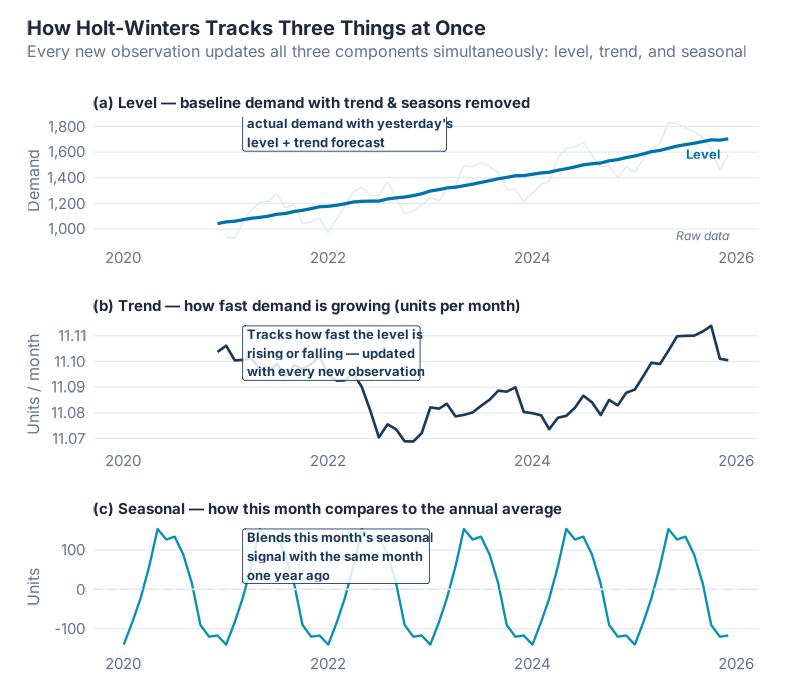
The profound elegance of the method is what each of these updates actually is: a weighted average between what the data just showed and what the model previously believed. New information is never ignored; old information is never fully overwritten. The three smoothing parameters — α, β, and γ — decide how fast the past fades. That is the philosophical heart of exponential smoothing, and you can understand everything important about it without a single formula.
The Three Dials: α, β, and γ
Each of the three components — level, trend, seasonal — has its own smoothing parameter. These are not arbitrary mathematical notations; they are genuinely meaningful controls you can reason about.
α — The Level Dial
α controls how quickly the model updates its estimate of the current baseline demand.
Think of it as a trust dial. Turn it up high (toward 1) and the model says: „I mostly trust what just happened — that last data point tells me a lot about where we are.“ Turn it down low (toward 0) and the model says: „One month doesn’t tell me much — I’m averaging over a long history to find the true level.“
A retail forecast that needs to respond quickly to a sudden demand shift would use a higher α. A stable industrial component with slow-moving demand would use a lower α — you want the model to be calm, not jumpy.
β — The Trend Dial
β controls how quickly the trend estimate is allowed to change direction.
High β means the model can „pivot“ on the trend quickly — if sales have been growing and suddenly flatten, the trend estimate bends fast. Low β means the trend is almost fixed for the life of the forecast — the model behaves as if it has a relatively stable long-term slope that won’t be thrown off by a few unusual months.
For most supply chain applications, β ends up quite low — 0.05 to 0.2. Real demand trends do not reverse overnight, and you do not want the model chasing every quarter’s deviation.
γ — The Seasonal Dial
γ controls whether the seasonal pattern is allowed to evolve over time.
High γ means December this year can look materially different from December last year — the model relearns the seasonal shape from recent data. Low γ means the seasonal pattern is treated as nearly fixed — December is December, and the model uses the long historical average of what December looks like.
For products where the seasonal swing is very stable (beer, certain pharmaceuticals), a low γ is natural. For fashion retail, where what „summer demand“ looks like can shift substantially from year to year, a higher γ gives the model more flexibility.
| Parameter | Controls | High value (≈ 1) | Low value (≈ 0) |
|---|---|---|---|
| α | Level responsiveness | Follows recent data closely; reacts fast to demand shifts | Heavily averaged; stable but slow to react |
| β | Trend flexibility | Trend can turn quickly; projects recent slope changes | Trend is nearly fixed; projects a stable long-run slope |
| γ | Seasonal flexibility | Seasonal shape evolves year to year | Seasonal shape is almost static |
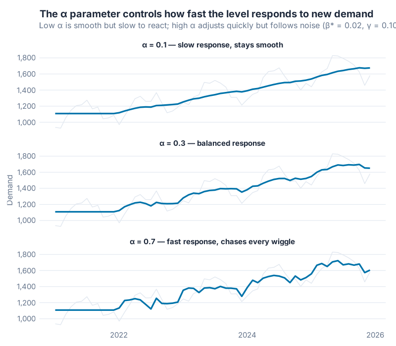
In a modern fpp3 workflow, you almost never set these by hand. You call ETS(), let the statistical model estimate them by maximum likelihood, and then check that the values look plausible. The report() function shows you exactly what the model chose and why. Most real-world series end up with α somewhere between 0.1 and 0.5 — moderate smoothing, not the extremes. If your estimated α is hugging 1.0, that is often a sign that your data has a structural break and the model is trying to cope by chasing every observation.
Additive vs. Multiplicative: Choosing the Right Seasonal Shape
This is the most practical choice you will make when applying Holt-Winters. The answer comes from simply looking at your data.
Additive seasonality means the seasonal swings stay roughly the same size regardless of where the overall level is. A warehouse that ships 200 extra pallets every December whether the baseline is 1,000 or 5,000 has additive seasonality — the December bump is a fixed amount.
Multiplicative seasonality means the seasonal swings scale with the level. A retailer where December is always about 30% above the monthly average — whether that average is €1 million or €10 million — has multiplicative seasonality. The December bump is a fixed ratio.
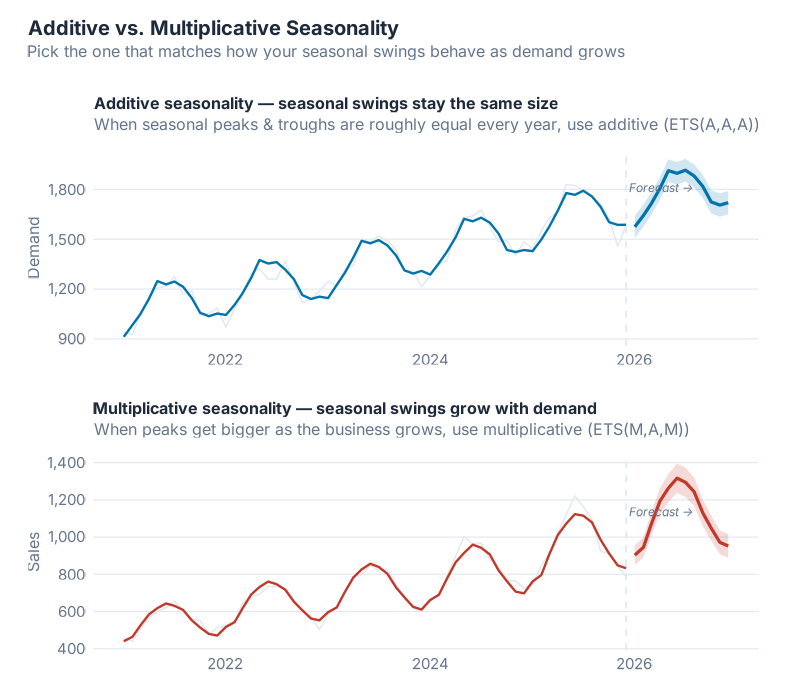
A quick rule of thumb for supply chain:
- Industrial and MRO demand tends to be additive — the seasonal uplift in June is a fixed quantity of parts, not a percentage of whatever you happen to be selling.
- Retail and consumer goods tends to be multiplicative — the Christmas uplift is a fraction of total volume, and as the brand grows, Christmas grows with it.
- When in doubt: look at whether the seasonal peaks get taller as the series trends upward. If yes, multiplicative. If the peaks stay about the same height through a rising trend, additive.
The good news: ETS() in fpp3 evaluates both and picks whichever fits better. You do not have to decide by hand unless you want to.
Damped Trend: The Fix That Saved Long-Horizon Forecasts
Here is the single most underappreciated improvement to exponential smoothing in the last forty years, and you can understand why it matters without a formula.
The problem: Undamped Holt-Winters projects its trend forward forever. If your model has learned that demand is growing by 150 units per month, it will project that same growth rate 6 months out, 12 months out, 24 months out, indefinitely. The forecast becomes a straight line shooting off into the future with total confidence. In theory this is elegant. In practice, it is how you end up overcommitting to production capacity you will never use.
The analogy: Imagine driving a car at 100 km/h on a highway and trying to predict where you will be in two hours. For the first 15 minutes, projecting your current speed forward is probably fine. But no sane navigator would project that speed forward two hours and mark the destination on a map, because they know you will slow down, stop for fuel, hit traffic, take an exit. Real-world trajectories don’t maintain their slope forever.
Undamped Holt-Winters is the navigator who marks the destination two hours away at exactly 100 km/h and calls it a day.
The fix: Gardner and McKenzie’s 1985 damped trend adds a single extra parameter — φ (phi) — that gently applies the brakes. At short horizons (1–3 months), the damped and undamped forecasts are nearly identical. At medium horizons (6–12 months), the damped forecast curves gradually toward a flat line, reflecting the realistic expectation that trends slow down. At long horizons (24+ months), the damped forecast levels off at a bounded value, while the undamped version keeps shooting upward.
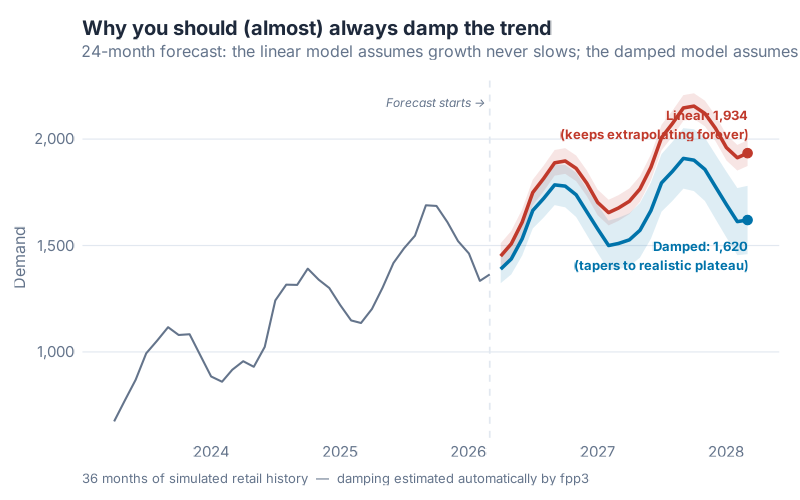
You do not need to understand the math of how φ works to appreciate the result: the damped forecast is a car coasting to a stop, not one accelerating forever. In the M3 and M4 forecasting competitions — the largest empirical comparisons of forecasting methods ever conducted — damped-trend variants of exponential smoothing consistently ranked among the top performers, often beating far more complex methods on monthly business data.
The practical takeaway: If you are forecasting more than about 12 periods ahead and your series has a trend, default to a damped model. In fpp3 notation, the trend component should be Ad (additive damped) or Md (multiplicative damped), not a plain A or M. ETS() considers damped models automatically, and in most medium-to-long horizon settings, it will pick one.
The ETS Framework: A Map of the Whole Method Family
One of the great contributions of the Hyndman-era state-space reframing was giving the entire exponential smoothing family a coherent naming scheme. Every variant gets a three-letter label: (Error, Trend, Seasonal).
- Error is either A (additive) or M (multiplicative)
- Trend is N (none), A (additive), Ad (additive damped), M (multiplicative), or Md (multiplicative damped)
- Seasonal is N (none), A (additive), or M (multiplicative)
Put those together and you get the whole family. The table below maps the common ones to the classical names you will recognize:
| ETS model | Classical name | Best for |
|---|---|---|
| ETS(A,N,N) | Simple exponential smoothing | No trend, no seasonality, stable level |
| ETS(A,A,N) | Holt’s linear method | Clear trend, no seasonality |
| ETS(A,Ad,N) | Damped Holt | Clear trend, no seasonality, medium/long horizon |
| ETS(A,A,A) | Additive Holt-Winters | Trend + seasonality, constant seasonal amplitude |
| ETS(A,Ad,A) | Damped additive Holt-Winters | Trend + seasonality, long horizon, stable amplitude |
| ETS(M,A,M) | Multiplicative Holt-Winters | Trend + seasonality, seasonal amplitude grows with level |
| ETS(M,Ad,M) | Damped multiplicative Holt-Winters | The workhorse for retail/consumer demand |
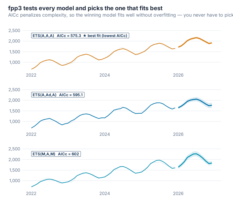
The practical move in fpp3: call ETS(Demand) with no model specification, and the function evaluates every admissible combination, fits each one by maximum likelihood, and picks the one with the lowest AICc. AICc (corrected Akaike Information Criterion) is a standard measure that balances fit quality against model complexity — exactly the right trade-off when your typical SKU has three years of monthly data and not much more.
You get the pedagogical clarity of the classical three-component method and the statistical discipline of modern model selection. Both, at the same time, from a single function call.
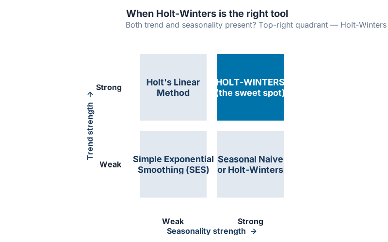
When Holt-Winters Shines
The Holt-Winters family is phenomenal on the exact kind of data most supply chain professionals work with every day:
- Strong trend combined with strong seasonality on a single annual or weekly cycle
- A single dominant seasonal period: monthly data with yearly seasonality, weekly data with quarterly seasonality, daily data with weekly seasonality
- Stable regime: no major structural breaks, no lost customers the size of your biggest one, no pandemic
- Short-to-medium forecast horizon: 1 to 24 periods, which is where almost all S&OP forecasting lives
- Need for interpretable outputs: you can show α, β, γ, and φ to a CFO and actually explain what they mean
That last bullet is the sleeper advantage. Modern machine-learning forecasts — neural networks, gradient boosters, Prophet with external regressors — can be impressively accurate, but they are opaque. When your forecast is wrong, „the model said so“ is not a satisfying answer to the person responsible for inventory planning. With ETS, you can point at a single number (say, α = 0.42) and say „the model weights the most recent month about 42% and the prior history about 58%, and it damps the trend by 2% per period.“ That level of interpretability is worth more than two percentage points of MAPE in most corporate contexts.
When Holt-Winters Fails
The method is not universal. These are the five situations where Holt-Winters will let you down, and what to use instead:
- Multiple seasonalities. Hourly retail traffic has a daily cycle (lunch rush), a weekly cycle (weekend vs weekday), and an annual cycle (Christmas). Classical Holt-Winters handles exactly one seasonal period at a time. Use TBATS or the MSTL + ETS hybrid instead.
- Structural breaks. ETS assumes the states evolve smoothly. A COVID-like shock — demand drops 60% in one month, returns six months later at a permanently higher level — is not a smooth evolution. ETS will chase the break, overshoot in both directions, and take 12–18 months to stabilize. Use regression with ARIMA errors and an intervention variable, or a Bayesian state-space model with a level-shift prior.
- Non-linear trends. S-curves, logistic growth, product launch ramps, EOL declines — Holt-Winters projects a straight (or gently curved) line. When the underlying process is sigmoidal, the straight line will be wrong at every part of the curve. Use Prophet with a logistic growth term.
- Intermittent demand. Slow-moving spare parts with many zero-demand months violate the ETS assumption that the level drifts smoothly. Use Croston’s method or its modern refinements (SBA, TSB), available in the
tsintermittentpackage. - Long horizons without damping. Already covered, but worth repeating: if you forecast more than 12 periods ahead without a damped trend, your prediction intervals will widen to comedy. Always damp for medium-to-long horizons.
Being honest about these failure modes is what separates a forecasting professional from a software demo. Holt-Winters is a scalpel, not a Swiss Army knife. When the job calls for a scalpel, nothing else is as clean. When it does not, a scalpel is actively dangerous.
The Modern ETS Workflow in R
In the fpp3 ecosystem — which is where every serious R-based supply chain forecaster should be working today — the whole Holt-Winters / ETS machinery collapses into a short, legible pipeline. You do not hand-code the three equations. You let the framework handle them.
The workflow has five steps:
- Fit —
model(ETS(Demand))evaluates every admissible ETS model and returns the AICc winner - Report —
report(fit)prints the chosen model, the estimated smoothing parameters, and the initial states - Inspect components —
components(fit)extracts the fitted level, trend, and seasonal states so you can see what the model thinks is going on inside your data - Diagnose residuals —
augment(fit)plusfeatures(.innov, ljung_box, lag = 24)checks whether the residuals look like white noise; if they do not, the model is missing something - Forecast —
forecast(fit, h = 12)returns point forecasts plus genuine prediction intervals derived from the fitted state-space model
The complete R script for everything in this post is in the collapsible section at the bottom.
Interactive Dashboard
The best way to build intuition for α, β, γ, and φ is to move them and watch the forecast respond. Pick one of four demand datasets (Retail Electronics, Spare Parts, Fashion Retail, or F&B with COVID shock). Drag the α slider and watch the fitted line hug every wiggle in the history. Switch from linear to damped trend on a 24-month forecast and watch the projection flatten out. Then click Let ETS pick α, β, γ, φ and see which model the likelihood-based AICc selection actually chooses — and how its holdout error stacks up against the one you just hand-tuned.
The key number on the dashboard is not the train RMSE. It is the holdout RMSE on the final 20% of the series, and the dashboard color-codes it: green when the holdout error stays close to the training error, red when it is more than 2.5× larger. Push α toward 0.9 on Retail Electronics and watch the Holdout KPI turn red in real time. This is the moment the three dials stop feeling like abstract parameters and start feeling like a tool you can control.
Interactive Dashboard
Explore the data yourself — adjust parameters and see the results update in real time.
Your Next Steps
Knowing the history is interesting. Knowing the concepts is satisfying. But the only thing that matters is whether you can make a better forecast tomorrow than you made today. Here are five concrete things to do this week:
- Fit
ETS()to your top-10 SKUs by revenue. Use at least three years of monthly history. Callreport()on each fitted model and write down the ETS triple it picked. You will immediately see patterns — most of your high-volume SKUs probably share the same structure, and the few that do not are the ones worth investigating. - Check your chosen α, β, γ values for sanity. If any parameter is pinned near 1.0 or near zero, something is off. An α near 1 usually means the series has a structural break the model is chasing. A γ near 0 means the seasonal pattern is static — fine, but verify visually. Large β values mean the trend is turning quickly, which may or may not be realistic for your product.
- Damp your long-horizon forecasts. If you are projecting more than twelve months out with any model that has a trend component, verify the trend is damped. In fpp3 this means the chosen model’s trend component should be
AdorMd, notAorM. If it is not, override withETS(Demand ~ trend("Ad"))and compare the two forecasts at the 24-month horizon. One of them is almost certainly more defensible than the other. - Run the Ljung-Box test on your residuals.
augment(fit) |> features(.innov, ljung_box, lag = 24)returns a p-value. If it is below 0.05, your residuals have autocorrelation left in them — the model is missing something. Common culprits: a second seasonal period, a structural break, or a trend pattern that the linear-ish ETS cannot capture. Fix what you can and refit. - Benchmark ETS against whatever your ERP is currently producing. Export the forecast your ERP generated for last quarter, pull the actuals, and compute MAPE or RMSE on both. Then do the same for an
ETS()forecast fit to the same history. On most demand series, the gap will be embarrassing for the ERP. That is your business case for putting an R script in the loop.
Show R Code
# =============================================================================
# Holt-Winters Exponential Smoothing — Complete Reproducible Code
# For "Holt-Winters Explained" blog post (inphronesys.com)
# =============================================================================
# Paste this into R or RStudio to reproduce all analyses from the article.
# Requires: install.packages("fpp3")
# =============================================================================

library(fpp3)

set.seed(42)


# =============================================================================
# PART 1: Create Simulated Demand Data
# =============================================================================
# Realistic monthly demand with upward trend + fixed seasonal pattern.
# Replace this section with your own data (see PART 7 below).

n <- 60  # 5 years of monthly data

t <- 1:n
seasonal_signal <- 150 * sin(2 * pi * t / 12 - pi / 2)   # annual cycle
demand_raw      <- 1000 + 12 * t + seasonal_signal + rnorm(n, sd = 40)

demand_ts <- tibble(
  Month  = yearmonth("2021 Jan") + 0:(n - 1),
  Demand = demand_raw
) |>
  as_tsibble(index = Month)

# Quick look at what we're working with
autoplot(demand_ts, Demand) +
  labs(title = "Monthly Demand — 5 Years of History",
       x = NULL, y = "Units")


# =============================================================================
# PART 2: Fit an ETS Model (Automatic Selection)
# =============================================================================
# ETS() with no constraints lets fpp3 search all valid combinations
# and pick the one with the lowest AICc (penalized goodness-of-fit).

fit <- demand_ts |>
  model(ETS(Demand))

# What model did it choose, and what are the smoothing parameters?
report(fit)

# The output shows:
#   ETS(A,A,A) = Additive errors, Additive trend, Additive season
#   alpha  = level smoothing  (high = react fast)
#   beta*  = trend smoothing  (typically small — trends change slowly)
#   gamma  = seasonal smoothing  (how fast seasonal pattern updates)
#   phi    = damping factor  (only present if trend is "Ad")


# =============================================================================
# PART 3: Inspect the Three State Variables
# =============================================================================
# components() extracts level, trend, and seasonal from the fitted model.

comp <- components(fit)
autoplot(comp) +
  labs(title = "ETS Components: Level, Trend, and Seasonal")

# Each panel shows one thing:
#   Level    — the baseline demand after removing trend and seasonality
#   Slope    — how fast the level is rising (or falling) right now
#   Seasonal — this month's typical deviation from the baseline


# =============================================================================
# PART 4: Check Fitted Values and Residuals
# =============================================================================
# augment() adds fitted values (.fitted) and residuals (.innov) to your data.
# Good residuals: look like random noise — no pattern, no autocorrelation.

aug <- augment(fit)
aug

# Visual residual check
aug |>
  autoplot(.innov) +
  labs(title = "Innovation Residuals — should look like white noise",
       y = "Residual")

# Formal residual check
fit |> gg_tsresiduals()


# =============================================================================
# PART 5: Forecast 12 Months Ahead with Prediction Intervals
# =============================================================================
# forecast() produces point forecasts + uncertainty bands.
# level = c(80, 95) gives 80% and 95% prediction intervals.

fc <- fit |>
  forecast(h = 12, level = c(80, 95))

# Plot with historical data in background
fc |>
  autoplot(demand_ts) +
  labs(title = "12-Month Forecast with Prediction Intervals",
       subtitle = "Shaded bands = 80% and 95% prediction intervals",
       x = NULL, y = "Units")

# Extract the numbers
fc |>
  as_tibble() |>
  select(Month, .mean) |>
  mutate(.mean = round(.mean)) |>
  print(n = 12)


# =============================================================================
# PART 6: Compare Damped vs. Undamped Trend
# =============================================================================
# The damped trend (Ad) prevents the model from forecasting forever upward.
# In practice, it almost always performs better on longer horizons.

fit_compare <- demand_ts |>
  model(
    Linear = ETS(Demand ~ error("A") + trend("A")  + season("A")),
    Damped = ETS(Demand ~ error("A") + trend("Ad") + season("A"))
  )

# AICc: lower = better fit (penalizes model complexity automatically)
glance(fit_compare) |>
  select(.model, AICc) |>
  arrange(AICc)

# 24-month forecast comparison
fc_compare <- fit_compare |>
  forecast(h = 24, level = 80)

fc_compare |>
  autoplot(demand_ts) +
  labs(title = "Damped vs. Linear Trend — 24-month horizon",
       subtitle = "Damped trend tapers to a realistic plateau; linear extrapolates forever",
       x = NULL, y = "Units")


# =============================================================================
# PART 7: Apply to Your Own Data
# =============================================================================
# Replace the block below with your actual data.
# All you need: a date column (monthly) and a numeric demand column.

# --- Option A: read from CSV ---
# your_data <- read.csv("your_file.csv") |>
#   mutate(Month = yearmonth(your_date_column)) |>
#   as_tsibble(index = Month)

# --- Option B: build from vectors ---
# your_months  <- yearmonth(seq(as.Date("2022-01-01"),
#                               as.Date("2024-12-01"), by = "month"))
# your_demand  <- c(420, 395, 440, ...)  # paste your values here
#
# your_data <- tibble(Month = your_months, Demand = your_demand) |>
#   as_tsibble(index = Month)

# Once you have your_data, the rest is identical:
# fit_yours <- your_data |> model(ETS(Demand))
# report(fit_yours)                       # what model was chosen?
# fit_yours |> forecast(h = 12) |>        # 12-month forecast
#   autoplot(your_data)
References
- Brown, R.G. (1956). Exponential Smoothing for Predicting Demand. Cambridge, Massachusetts: Arthur D. Little.
- Brown, R.G. (1959). Statistical Forecasting for Inventory Control. New York: McGraw-Hill.
- Holt, C.C. (1957). Forecasting Seasonals and Trends by Exponentially Weighted Moving Averages. Office of Naval Research Memorandum No. 52, Carnegie Institute of Technology. Reprinted in Holt, C.C. (2004), „Forecasting seasonals and trends by exponentially weighted moving averages,“ International Journal of Forecasting, 20(1), 5–10.
- Winters, P.R. (1960). Forecasting Sales by Exponentially Weighted Moving Averages. Management Science, 6(3), 324–342.
- Gardner, E.S., Jr., & McKenzie, E. (1985). Forecasting Trends in Time Series. Management Science, 31(10), 1237–1246.
- Hyndman, R.J., Koehler, A.B., Snyder, R.D., & Grose, S. (2002). A state space framework for automatic forecasting using exponential smoothing methods. International Journal of Forecasting, 18(3), 439–454.
- Hyndman, R.J., Koehler, A.B., Ord, J.K., & Snyder, R.D. (2008). Forecasting with Exponential Smoothing: The State Space Approach. Berlin: Springer-Verlag.
- Hyndman, R.J., & Athanasopoulos, G. (2021). Forecasting: Principles and Practice, 3rd edition. OTexts. Chapter 8: Exponential Smoothing.
- Gardner, E.S., Jr. (2006). Exponential smoothing: The state of the art — Part II. International Journal of Forecasting, 22(4), 637–666.
- Makridakis, S., Spiliotis, E., & Assimakopoulos, V. (2020). The M4 Competition: 100,000 time series and 61 forecasting methods. International Journal of Forecasting, 36(1), 54–74.
Schreibe einen Kommentar