Most supply chain professionals can name three forecasting methods. Almost none can name the three people who invented them. We spend careers arguing about ETS versus Prophet, Holt-Winters versus gradient boosting, without ever knowing whose shoulders we are standing on — or who is still shaping where the field goes next.
Here is the fix. Twenty people. Five categories. One "start here" resource per person. If you follow, read, and listen to this list over the next six months, you will learn more about demand planning, probabilistic thinking, and modern ML forecasting than any single textbook can teach you. Consider it a syllabus disguised as a TIME 100.
Two axes: academic ↔ practitioner and classical stats ↔ ML. Dot size reflects editorial read of reach — not a ranking. Five categories fell out naturally: Academics who set the theoretical foundations, Decision Scientists who study how humans forecast, ML Builders shipping the tools practitioners actually use, Supply Chain Voices translating theory into S&OP rooms, and Popularizers who made probabilistic thinking mainstream.
The Forecasting Landscape
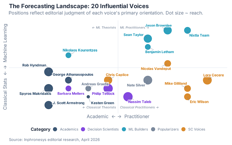
Two things stand out when you see them plotted together. First, the ML frontier is clustered in the top-right — Nixtla, Jason Brownlee, Sean Taylor — but the people bridging classical stats and ML (Nikolaos Kourentzes, Nicolas Vandeput) sit closer to the middle and are arguably the most useful to a supply chain reader. Second, the highest-reach voices (the big dots — Tetlock, Taleb, Cecere, Silver) are almost all in the right half. Popularity follows practitioners, not theorists. Worth remembering when you wonder why Hyndman’s book is free on the internet.
The Academics: Where the Math Comes From
These five are why your forecasting software has the options it has. When Excel offers you "exponential smoothing" or your R package prints out an ARIMA(2,1,2), that menu was shaped by their research. You do not need to read their papers to be a good forecaster — but reading one of them will change how you read every vendor pitch for the rest of your career.
Rob Hyndman
Professor of Statistics at Monash University and the most widely read forecasting educator alive. He wrote the forecast and fable R packages that power a large chunk of academic and corporate time-series work, and made the definitive textbook available for free online. If you read only one thing from this entire list, read Hyndman.
Best resource: Forecasting: Principles and Practice (FPP3) — a free, chapter-by-chapter walkthrough of everything from naïve benchmarks to hierarchical reconciliation, with runnable R code throughout.
Spyros Makridakis
Professor at the University of Nicosia and the architect of the M-Competitions (M1 through M6) — the running empirical tournament that answers the only forecasting question that matters: which methods actually work? Makridakis’s finding that simple models frequently beat complex ones is the most inconvenient truth in the field.
Best resource: The M4 Competition: Results, Findings, Conclusion — a short, readable paper that will make you skeptical of anyone selling "sophisticated" forecasts without a benchmark.
J. Scott Armstrong (1937–2023)
Professor Emeritus at Wharton and editor of Principles of Forecasting — the field’s compendium of what decades of research actually tell us about doing this well. Champion of judgmental forecasting, combining methods, and evidence-based practice long before "evidence-based" was a buzzword. Armstrong passed away in September 2023, but his work remains foundational.
Best resource: Principles of Forecasting — dense, but the section on combining forecasts alone will pay for the read.
George Athanasopoulos
Professor at Monash and co-author of FPP3 with Hyndman. His research on hierarchical forecasting and reconciliation is the reason modern demand-planning tools can forecast SKU-level and country-level demand and actually have them add up.
Best resource: Forecasting: Principles and Practice (FPP3) — the chapters on hierarchical and grouped forecasting are his signature contribution.
Kesten Green
Associate Professor at the University of South Australia and co-maintainer of forecastingprinciples.com with Armstrong. His research on Structured Analogies — a disciplined way to forecast from similar past situations — showed the method beat unaided expert judgment roughly 60% to 32% on accuracy. The kicker: the technique takes one page to explain and is perfect for new-product launches where you have no history.
Best resource: forecastingprinciples.com — a curated reference site organized around evidence-based rules rather than techniques.
The Decision Scientists: How Humans Actually Forecast
Statistics is about models. Decision science is about minds. These three changed how serious people think about uncertainty, calibration, and the limits of prediction — which matters because every S&OP meeting ever held is really a decision-science problem, not a statistics problem.
Philip Tetlock
Professor at Wharton and the researcher behind the Good Judgment Project, which showed that a small group of trained amateurs — "superforecasters" — consistently outperformed U.S. intelligence analysts on geopolitical questions. If you have ever sat through a forecast review and thought "these people sound way too confident," Tetlock explains why.
Best resource: Superforecasting: The Art and Science of Prediction — a readable, non-technical book that has more practical advice for running a demand planning meeting than most SCM textbooks.
Barbara Mellers
Professor of Psychology at Penn and co-lead of the Good Judgment Project with Tetlock. Her research on how training, feedback, and aggregation improve probabilistic judgment is the academic backbone of everything the superforecasting movement claims.
Best resource: Psychological Strategies for Winning a Geopolitical Forecasting Tournament — a short paper that reads like an operations manual for running better forecast reviews.
Nassim Taleb
Distinguished Professor of Risk Engineering at NYU Tandon and the person who made "tail risk" a phrase supply chain people actually use. Love him or disagree with him, The Black Swan permanently changed how serious planners think about rare, high-impact events — which is to say, every disruption that has mattered in the last decade.
Best resource: The Black Swan — read it once, remember it every time someone asks you for a "point forecast" of something inherently uncertain.
The ML Builders: The Tools You Actually Use
If the Academics gave the field its menu, the ML Builders gave it the kitchen. These are the people whose open-source packages are running inside your demand-planning workflow right now, whether you know it or not.
Sean Taylor
Chief Scientist at Motif Analytics, previously at Meta and Lyft, and co-creator of Prophet — the forecasting library that introduced an entire generation of data scientists to time series because pip install prophet worked on the first try. Writes thoughtfully on causal inference and forecasting workflows.
Best resource: Prophet — the docs are a surprisingly good forecasting tutorial in their own right.
Benjamin Letham
Research Scientist at Meta and co-creator of Prophet with Taylor. He designed the Bayesian changepoint-detection mechanism that lets Prophet automatically find regime shifts in a time series — the single feature most responsible for Prophet’s "just works" reputation on messy business data. He is also a core contributor to BoTorch, Meta’s open-source Bayesian optimization library.
Best resource: Forecasting at Scale (Prophet paper) — the short paper that explains exactly what Prophet is doing under the hood. Read it before you trust Prophet in production.
Max Mergenthaler Canseco
Co-founder of Nixtla, the open-source company behind StatsForecast, MLForecast, NeuralForecast, and TimeGPT — the fastest-growing Python forecasting stack. Their libraries have dominated recent M-competition benchmarks and made high-quality statistical forecasting an import away.
Best resource: StatsForecast — start here even if you think you are an "ML person"; their classical implementations are faster and more accurate than most ML alternatives.
Nikolaos Kourentzes
Professor at the University of Skövde and the most useful bridge voice in the field — he understands classical stats deeply, works on neural nets for forecasting, and writes about both clearly. His research on temporal hierarchies is quietly reshaping how long-range plans are built.
Best resource: kourentzes.com forecasting blog — practitioner-oriented posts that translate research into things you can actually do on Monday.
Jason Brownlee
Founder of Machine Learning Mastery and, for better or worse, how a large share of working ML practitioners first learned Python. His "Introduction to Time Series Forecasting" tutorials are the path from "I know pandas" to "I can train an LSTM on demand data" for thousands of analysts.
Best resource: Machine Learning Mastery — start with the time series tutorials; they are not academic, and that is the point.
The Supply Chain Voices: Where the Forecasts Actually Land
Forecasts live or die in the S&OP meeting. These five are the people translating everything above into language that planners, procurement leads, and CFOs can use. If you work in supply chain, this is the group you should be following hardest on LinkedIn.
Mike Gilliland
Author of The Business Forecasting Deal, former SAS forecasting practice lead, and the person who made Forecast Value Added (FVA) a standard metric. The first writer to take seriously the inconvenient question: "is our forecasting process actually making forecasts better, or is it just expensive theater?"
Best resource: The Business Forecasting Deal — equal parts diagnosis of bad forecasting process and playbook for fixing it.
Nicolas Vandeput
Supply chain data scientist, founder of SupChains, and author of Data Science for Supply Chain Forecasting and Demand Forecasting Best Practices. One of the few people writing in the sweet spot between "I can read a Jupyter notebook" and "I run a demand planning team."
Best resource: Demand Forecasting Best Practices — the SCM-focused companion to Hyndman that a lot of practitioners wish they had started with.
Chris Caplice
Executive Director of the MIT Center for Transportation & Logistics and the force behind the MIT MicroMasters in Supply Chain Management — the gold-standard online SCM program. Has personally introduced tens of thousands of working professionals to forecasting and analytics.
Best resource: MIT MicroMasters: Supply Chain Management — if you want a credential that recruiters and peers both respect, this is the one.
Lora Cecere
Founder of Supply Chain Insights and, with roughly 348,000 LinkedIn followers, the most-followed supply chain voice on the platform. Relentlessly skeptical of vendor narratives and steady advocate for outside-in, demand-driven thinking. If LinkedIn’s "Top Voice" in SCM had always existed, she would already have the badge.
Best resource: Supply Chain Insights — worth following for the vendor-honesty alone.
Eric Wilson
Director of Thought Leadership at the Institute of Business Forecasting & Planning (IBF) and the voice behind the IBF’s podcast and webinar output. A steady source of practitioner-to-practitioner conversations about S&OP, demand planning, and forecasting in the wild — not consultants pitching frameworks.
Best resource: IBF On Demand — bimonthly IBF podcast of practitioner-to-practitioner conversations with people actually running planning functions.
The Popularizers: The On-Ramps
Two voices you can use to pull colleagues into probabilistic thinking before they ever hear the word "ETS." The popularizer slot is small because the job is hard — making forecasting interesting to non-forecasters without losing the math.
Nate Silver
Statistician, author, and founder of FiveThirtyEight (now writing at Silver Bulletin). The Signal and the Noise is the most widely read forecasting book outside academia, which is why you keep meeting non-specialists who suddenly understand what a probability distribution is.
Best resource: The Signal and the Noise — the one book to hand to a colleague who says "forecasts are always wrong" and means it as a serious argument.
Andreas Graefe
Professor at Macromedia University. If combining five forecast methods and averaging the result sounds obvious, credit Graefe: his PollyVote research was the first to quantify how much combining actually helps — roughly 5% to 41% error reduction versus any single model, depending on how different the methods are. Every ensemble you run in your demand-planning tool traces back to this line of work.
Best resource: PollyVote — read the methodology page; it is a mini-lecture on why combining forecasts works.
The Resource Shelf
If you are not going to follow twenty people, follow ten resources. These are the ten starting points we would put on a single shelf, scored on a combination of accessibility and impact.
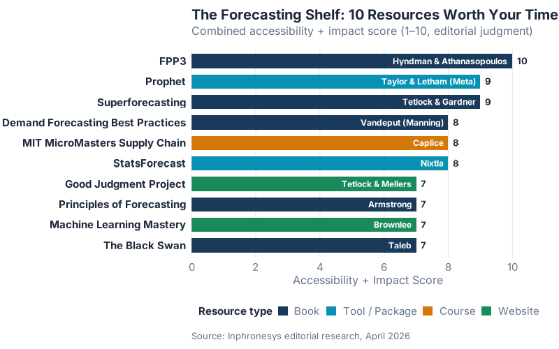
Two patterns worth noticing. First, the top of the shelf is free — FPP3, Prophet docs, StatsForecast docs, the Good Judgment site. Cost is not the bottleneck in learning to forecast; attention is. Second, the ranking mixes books, tools, courses, and websites on purpose. Different formats stick for different people, and a planner who never reads a textbook but works through the Prophet Quickstart is not a worse forecaster than one who finishes FPP3 chapter by chapter.
Your Learning Path
Do not try to drink from all 20 firehoses. Pick one row based on where you sit today.
| Level | Start With | Then | Go Deeper |
|---|---|---|---|
| Beginner | Superforecasting — to fix your intuition about uncertainty first | FPP3 chapters 1–5 — naïve benchmarks, simple methods, ETS | Demand Forecasting Best Practices — apply it to your actual SKUs |
| Intermediate | StatsForecast — run the tutorial on your own data this week | FPP3 chapters 6–11 — ARIMA, hierarchical, judgmental adjustments | M4 Competition paper — so you stop trusting complexity without a benchmark |
| Advanced | Principles of Forecasting — the combining-forecasts sections | Kourentzes’s blog + Prophet paper — modern bridges | The Business Forecasting Deal — because at your level the hard problem is process, not math |
The one rule: finish each step before starting the next. Half-reading FPP3 and half-watching a Nixtla tutorial is worse than finishing either one.
Interactive Dashboard
Explore all 20 profiles yourself — filter by category, focus area, or learning level, search by name, and build a personalized reading list you can save for later.
Interactive Dashboard
Explore the data yourself — adjust parameters and see the results update in real time.
Your Next Steps This Week
- Today: pick one person from this list who is not already in your feed and follow them on LinkedIn or subscribe to their newsletter.
- This week: read one chapter of FPP3 — chapter 5 ("The forecaster’s toolbox") is the single most useful starting point.
- This month: run the StatsForecast tutorial on one of your own SKUs and benchmark it against your current forecast.
- This quarter: either finish Superforecasting or watch one block of the MIT MicroMasters — both will change how you sit in your next S&OP meeting.
- This year: pick two voices from the list above and actually engage with them — comment on their posts, ask a question, send an email. The forecasting community is small, and most of these people reply.
Which of these 20 has already shaped how you forecast, and what did they teach you? (And who would you add?) Drop a comment — we will update the map in a future post based on who you bring to the conversation.
Show R Code
# =============================================================================
# generate_whos_who_images.R
# Produces two images for the "Who's Who in Forecasting" blog post:
#   1. ww_influence_map.png      — 2D scatter of 20 influential voices
#   2. ww_resource_shelf.png     — horizontal bar chart of 10 learning resources
# =============================================================================

source("Scripts/theme_inphronesys.R")

library(ggplot2)
library(dplyr)
library(ggrepel)
library(scales)

set.seed(42)

# -----------------------------------------------------------------------------
# Category color map (explicit per task brief)
# -----------------------------------------------------------------------------
cat_colors <- c(
  "Academics"           = iph_colors$navy,
  "Decision Scientists" = "#6d28d9",                # purple
  "ML Builders"         = iph_colors$teal,
  "SC Voices"           = iph_colors$orange,
  "Popularizers"        = iph_colors$grey
)

# -----------------------------------------------------------------------------
# Data: 20 influential voices
# x: Academic (1) <-> Practitioner (10)
# y: Classical Stats (1) <-> Machine Learning (10)
# size: influence / reach (1–10, bigger = more widely followed)
# -----------------------------------------------------------------------------
people <- tibble::tribble(
  ~name,                    ~category,             ~x, ~y, ~size,
  "Rob Hyndman",            "Academics",            2,  5,  9,
  "Spyros Makridakis",      "Academics",            2,  3,  9,
  "J. Scott Armstrong",     "Academics",            2,  1,  8,
  "George Athanasopoulos",  "Academics",            3,  4,  6,
  "Kesten Green",           "Academics",            4,  2,  4,
  "Philip Tetlock",         "Decision Scientists",  5,  3,  10,
  "Barbara Mellers",        "Decision Scientists",  3,  3,  5,
  "Nassim Taleb",           "Decision Scientists",  6,  2,  10,
  "Sean Taylor",            "ML Builders",          7,  9,  8,
  "Benjamin Letham",        "ML Builders",          7,  8,  5,
  "Nixtla Team",            "ML Builders",          9, 10,  6,
  "Nikolaos Kourentzes",    "ML Builders",          3,  7,  5,
  "Jason Brownlee",         "ML Builders",          8, 10,  8,
  "Mike Gilliland",         "SC Voices",            9,  3,  6,
  "Nicolas Vandeput",       "SC Voices",            8,  6,  6,
  "Chris Caplice",          "SC Voices",            5,  4,  8,
  "Lora Cecere",            "SC Voices",           10,  4,  9,
  "Eric Wilson",            "SC Voices",            9,  2,  6,
  "Nate Silver",            "Popularizers",         7,  4,  9,
  "Andreas Graefe",         "Popularizers",         4,  3,  5
)

# -----------------------------------------------------------------------------
# Plot 1 — The Forecasting Landscape (Influence Map)
# -----------------------------------------------------------------------------
p1 <- ggplot(people, aes(x = x, y = y)) +
  # Faint quadrant reference lines
  geom_hline(yintercept = 5.5, color = iph_colors$lightgrey, linewidth = 0.4) +
  geom_vline(xintercept = 5.5, color = iph_colors$lightgrey, linewidth = 0.4) +

  # Corner annotations — quadrant labels (inset so they don't hit axis/labels)
  annotate("text", x = 5.4, y = 10.5, label = "\u2190 ML Theorists",
           hjust = 1, vjust = 1, size = 3.0, fontface = "italic",
           color = iph_colors$grey) +
  annotate("text", x = 5.6, y = 10.5, label = "ML Practitioners \u2192",
           hjust = 0, vjust = 1, size = 3.0, fontface = "italic",
           color = iph_colors$grey) +
  annotate("text", x = 5.4, y = 0.6, label = "\u2190 Classical Theorists",
           hjust = 1, vjust = 0, size = 3.0, fontface = "italic",
           color = iph_colors$grey) +
  annotate("text", x = 5.6, y = 0.6, label = "Classical Practitioners \u2192",
           hjust = 0, vjust = 0, size = 3.0, fontface = "italic",
           color = iph_colors$grey) +

  geom_point(aes(color = category, size = size), alpha = 0.85) +

  geom_label_repel(
    aes(label = name, color = category),
    size = 3.1,
    family = "Inter",
    fontface = "bold",
    label.size = 0,
    label.padding = unit(0.15, "lines"),
    fill = alpha("white", 0.75),
    box.padding = 0.45,
    point.padding = 0.3,
    min.segment.length = 0.2,
    segment.color = iph_colors$grey,
    segment.alpha = 0.5,
    max.overlaps = Inf,
    seed = 42,
    show.legend = FALSE
  ) +

  scale_color_manual(values = cat_colors, name = "Category") +
  scale_size_continuous(range = c(3, 10), guide = "none") +
  scale_x_continuous(
    breaks = NULL,
    limits = c(0.5, 10.5)
  ) +
  scale_y_continuous(
    breaks = NULL,
    limits = c(0.5, 10.7)
  ) +
  labs(
    title    = "The Forecasting Landscape: 20 Influential Voices",
    subtitle = "Positions reflect editorial judgment of each voice's primary orientation. Dot size ~ reach.",
    x = "Academic  \u2190 \u2192  Practitioner",
    y = "Classical Stats  \u2190 \u2192  Machine Learning",
    caption = "Source: Inphronesys editorial research, April 2026"
  ) +
  theme_inphronesys(grid = "none") +
  theme(
    legend.position = "bottom",
    legend.title = element_text(face = "bold"),
    legend.text = element_text(size = 9),
    legend.key.size = unit(0.6, "lines"),
    legend.spacing.x = unit(0.2, "cm"),
    plot.margin = margin(10, 12, 8, 8)
  ) +
  guides(color = guide_legend(override.aes = list(size = 4, label = ""), nrow = 1))

ggsave(
  filename = "https://inphronesys.com/wp-content/uploads/2026/04/ww_influence_map-1.png",
  plot = p1,
  width = 8, height = 5, dpi = 100, bg = "white"
)

# -----------------------------------------------------------------------------
# Plot 2 — The Forecasting Shelf (Resource Bar Chart)
# -----------------------------------------------------------------------------
resource_colors <- c(
  "book"    = iph_colors$navy,
  "tool"    = iph_colors$teal,
  "course"  = iph_colors$orange,
  "website" = iph_colors$green
)

resources <- tibble::tribble(
  ~resource,                                              ~creator,                   ~type,     ~score,
  "FPP3",                                                 "Hyndman & Athanasopoulos", "book",    10,
  "Superforecasting",                                     "Tetlock & Gardner",        "book",     9,
  "Prophet",                                              "Taylor & Letham (Meta)",   "tool",     9,
  "StatsForecast",                                        "Nixtla",                   "tool",     8,
  "MIT MicroMasters Supply Chain",                        "Caplice",                  "course",   8,
  "Demand Forecasting Best Practices",                    "Vandeput (Manning)",       "book",     8,
  "The Black Swan",                                       "Taleb",                    "book",     7,
  "Machine Learning Mastery",                             "Brownlee",                 "website",  7,
  "Principles of Forecasting",                            "Armstrong",                "book",     7,
  "Good Judgment Project",                                "Tetlock & Mellers",        "website",  7
) |>
  mutate(
    resource = factor(resource, levels = resource[order(score, decreasing = FALSE)])
  )

p2 <- ggplot(resources, aes(x = score, y = resource, fill = type)) +
  geom_col(width = 0.7) +

  # Creator annotations — inside bar, right-aligned in white
  geom_text(
    aes(label = creator, x = score - 0.15),
    hjust = 1, color = "white", size = 3.1,
    family = "Inter", fontface = "bold"
  ) +

  # Score annotation at end of bar
  geom_text(
    aes(label = score, x = score + 0.15),
    hjust = 0, color = iph_colors$dark, size = 3.3,
    family = "Inter", fontface = "bold"
  ) +

  scale_fill_manual(
    values = resource_colors,
    name = "Resource type",
    breaks = c("book", "tool", "course", "website"),
    labels = c("Book", "Tool / Package", "Course", "Website")
  ) +
  scale_x_continuous(
    limits = c(0, 11),
    breaks = seq(0, 10, by = 2),
    expand = c(0, 0)
  ) +
  labs(
    title = "The Forecasting Shelf: 10 Resources Worth Your Time",
    subtitle = "Combined accessibility + impact score (1\u201310, editorial judgment)",
    x = "Accessibility + Impact Score",
    y = NULL,
    caption = "Source: Inphronesys editorial research, April 2026"
  ) +
  theme_inphronesys(grid = "x") +
  theme(
    legend.position = "bottom",
    axis.text.y = element_text(color = iph_colors$dark, face = "bold"),
    plot.margin = margin(10, 15, 8, 8)
  )

ggsave(
  filename = "https://inphronesys.com/wp-content/uploads/2026/04/ww_resource_shelf-1.png",
  plot = p2,
  width = 8, height = 5, dpi = 100, bg = "white"
)

cat("Generated: https://inphronesys.com/wp-content/uploads/2026/04/ww_influence_map-1.png\n")
cat("Generated: https://inphronesys.com/wp-content/uploads/2026/04/ww_resource_shelf-1.png\n")
References
- Hyndman, R. J., & Athanasopoulos, G. (2021). Forecasting: Principles and Practice (3rd ed.). OTexts. otexts.com/fpp3
- Makridakis, S., Spiliotis, E., & Assimakopoulos, V. (2020). The M4 Competition: 100,000 time series and 61 forecasting methods. International Journal of Forecasting, 36(1), 54–74. Link
- Armstrong, J. S. (Ed.). (2001). Principles of Forecasting: A Handbook for Researchers and Practitioners. Kluwer. Link
- Tetlock, P. E., & Gardner, D. (2015). Superforecasting: The Art and Science of Prediction. Crown. Link
- Mellers, B., et al. (2014). Psychological Strategies for Winning a Geopolitical Forecasting Tournament. Psychological Science, 25(5), 1106–1115. Link
- Taleb, N. N. (2010). The Black Swan (2nd ed.). Random House. Link
- Taylor, S. J., & Letham, B. (2017). Forecasting at scale. PeerJ Preprints. Link
- Gilliland, M. (2010). The Business Forecasting Deal. Wiley. Link
- Vandeput, N. (2023). Demand Forecasting Best Practices. Manning. Link
- Silver, N. (2012). The Signal and the Noise. Penguin Press. Link
Schreibe einen Kommentar