The agent looked like a star. Its suppliers would disagree.
Here is the pitch every vendor is making this year: stop hand-tuning reorder points, hand the replenishment decision to an AI agent, and let it react to demand in real time. It sounds great. The agent never sleeps, never forgets a SKU, never rounds a forecast down because it’s Friday.
So I built one and gave it the button.
In a 250-day simulation of a single SKU, the agent posted a fill rate of roughly 100%. It lost about 4 units of demand across the whole measured window. On its own scorecard it crushed the static reorder-point planner that most ERP systems ship with. If you stopped reading the report there, you’d promote it.
Then I looked one link upstream. The agent had taken a demand stream with a variance of 451 and turned it into an order stream with 6.65 times that variance. Same shelf, same service, and a firehose of noise pointed straight at every supplier behind it.
The danger of an agentic reorder system isn’t that it’s dumb. It’s that it’s too responsive. Give it the button with no guardrails and it will faithfully rebuild the one thing supply chain managers have spent thirty years trying to kill: the bullwhip effect.
What the agent is actually deciding
Strip the marketing away and a reorder agent does one thing each day: it picks an order quantity. Almost every sensible version targets an order-up-to level (a base-stock target). The logic is simple. Estimate demand, estimate variability, set a target stock position that covers the lead time plus a safety buffer, then order the gap between where you are and where you want to be.
The formula behind the target looks like this:
S = forecast × (L + 1) + z × σ × √(L + 1)
L is the lead time. z is the safety factor (1.65 here, for about 95% cycle service). σ is the demand standard deviation. Nothing exotic. The whole fight is over two words: which forecast, and how fast you let it move.
I ran three policies against identical demand. Same SKU. Same 5-day lead time. Same lost-sales rule (unmet demand walks out the door, it does not wait in a backlog). Same costs. Same random seed.
| Policy | How it sets the target | Reaction speed |
|---|---|---|
| Static planner | Fixed mean and sigma, set once | None |
| Naive agent | 3-day moving-average forecast, no limits | Maximum |
| Guardrailed agent | Smoothed forecast, dampened order, hard cap | Throttled |
The static planner is the human baseline: the reorder point you set in the ERP and forget. The naive agent is the literal "give the LLM the button" case. The guardrailed agent has the same autonomy and chases the same target, with three brakes bolted on. Those brakes are the whole story.
The demand I threw at them
Daily demand averaged 100 units with a weekly rhythm and a healthy dose of noise. Then, on day 150, I changed the world: a permanent step up of +30 units per day. A new customer, a won tender, a competitor exiting. Pick your reason. Demand never came back down.
That single shift is what separates a policy that works from a policy that just looks calm. Over the evaluation window (days 31 to 250, after a warm-up), demand ran at a mean of 113.3 units/day with a variance of 451.3. Everything below is measured on that window.
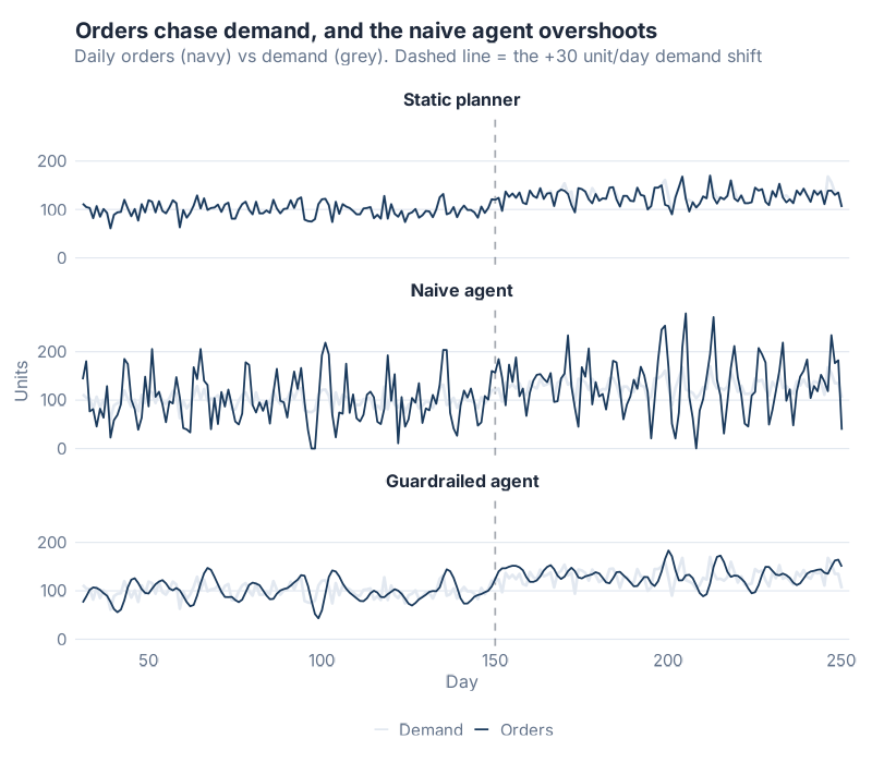
Look at the middle panel. The grey line is demand, doing what demand does. The navy line is the naive agent’s orders, and it has come unstuck from reality. The agent’s orders swing from zero to over 250 units in a single day, chasing a 3-day average that jerks around with every random bump. The static planner (top) barely moves. The guardrailed agent (bottom) tracks demand without the convulsions.
What jumped out at me wasn’t the day-150 step. All three policies eventually climb to the new level. It was the texture. The naive agent manufactures violence out of ordinary noise.
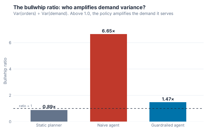
The one number that matters: bullwhip ratio
There’s a clean way to measure this. The bullwhip ratio is the variance of orders divided by the variance of demand. Above 1.0, a policy is amplifying: it sends its supplier more chaos than it received. Below 1.0, it’s absorbing, or under-reacting. Lee, Padmanabhan and Whang named this effect in 1997, and Chen et al. proved in 2000 that any order-up-to policy with a moving-average forecast amplifies by at least 1 + 2L/p + 2L²/p². That bound assumes idealized AR(1) demand, so it points to the direction, not the exact multiple my richer simulation produces. The lesson holds either way: short forecast window, long lead time, big amplification. The naive agent is that inequality walking around in a hoodie.
Here’s what each policy did to the demand variance:
| Policy | Bullwhip ratio |
|---|---|
| Static planner | 0.89× |
| Naive agent | 6.65× |
| Guardrailed agent | 1.47× |
The naive agent amplified demand variance 6.65×. The guardrailed agent: 1.47×. That’s 4.5× less noise dumped on suppliers, and it removes 78% of the amplification. Same agent autonomy. Same base-stock logic. The only difference is three lines of restraint.
The surprise: guardrails cost nothing
This is the part I didn’t expect, and it’s why I think the "more autonomy is always better" crowd has it backwards.
If guardrails throttled the agent, you’d expect to pay for them in service or stock. You don’t. The naive and guardrailed agents delivered identical service (both round to ~100% fill, 99.99% versus 100.0%) and near-identical inventory (168 versus 166 units) at near-identical total cost ($27,149 versus $27,056). The guardrailed version is actually a hair cheaper.
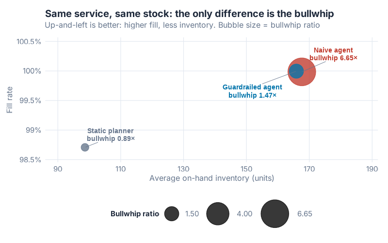
The two agent bubbles land in nearly the same spot: high fill, similar inventory. The naive agent’s bubble is just enormous, because bubble size is the bullwhip, and that’s the one axis where they diverge. You buy a 4.5× reduction in upstream noise for free. No service hit. No inventory penalty. The guardrails aren’t a trade-off. They’re a strict upgrade.
So why does the naive agent amplify so hard? It forecasts off a 3-day window, so a couple of high-demand days yank its forecast up. Then the (L + 1) multiplier on that jumpy forecast magnifies the move sixfold into the order. Next week it overshot, so it slams the order to zero. Chase, overshoot, slam, repeat. The agent isn’t malfunctioning. It’s doing exactly what you told it: react to the latest demand, fast.
The static planner isn’t the hero either
You might read all this and conclude the calm old static planner was right all along. Its bullwhip ratio is the lowest of the three: 0.89×. It under-amplifies. Suppliers love it.
That number is a halo on a corpse.
The static planner kept the leanest inventory (99 units) by ignoring the world. When demand stepped up on day 150, its fixed target never moved, so it lost 322 units of demand and stocked out on 20 of 220 days. Its fill rate fell to 98.7%, and its stockout penalty bill ran to $2,576 against the naive agent’s $31. Its orders are smoother than demand only because they’re deaf to it. A low bullwhip earned by failing to serve customers is not a win. It’s a different failure mode wearing better PR.
Here’s the full scorecard. Read it across, not down.
| Metric | Static planner | Naive agent | Guardrailed agent |
|---|---|---|---|
| Fill rate | 98.7% | ~100% | ~100% |
| Avg on-hand inventory | 99 units | 168 units | 166 units |
| Stockout days | 20 | 3 | 1 |
| Units of demand lost | 322 | ~4 | ~1 |
| Total cost | $22,226 | $27,149 | $27,056 |
| Bullwhip ratio | 0.89× | 6.65× | 1.47× |
The static planner wins on raw cost, but only because lost sales are cheap in this model ($8 a unit) and it never carries stock for demand it refuses to see. Raise the cost of a stockout, or care about your customers, and that $22,226 evaporates. The two agents are the real contest, and the guardrailed one wins it without giving anything up.
Where this breaks
A simulation is a clean room, and the real warehouse is not. Three honest limits.
First, this is one SKU with Gaussian-ish demand and a single clean step change. Intermittent or lumpy demand (the kind where SBA and Croston earn their keep) would punish the naive agent’s short window even harder, but the exact ratios would shift. Second, I assumed a fixed 5-day lead time. Variable lead times add their own variance, and a reactive agent tends to compound it. Third, the bullwhip ratio measures noise exported, not dollars lost upstream. A supplier with flexible capacity shrugs off a 6.65× ratio; one running lean chokes on it. The metric is a smoke alarm, not a damage estimate.
None of that rescues the naive agent. If anything, the messier real world makes its over-reaction more expensive, not less.
The bullwhip is someone else’s invoice
Put a number on it. If this SKU’s supplier sizes capacity and safety stock against the order variance it receives, the naive agent is asking that supplier to plan for a world with 6.65× the volatility that actually exists. That’s overtime, expedite fees, and bloated upstream safety stock, all to absorb noise a downstream algorithm invented. The guardrailed agent asks the same supplier to plan for 1.47×. Multiply across a few hundred SKUs and a multi-tier chain, and the bullwhip you let an agent generate at the buying desk becomes someone else’s capital tied up three tiers up.
The fix is not less AI. It’s three guardrails, and you can specify them in a sentence: smooth the forecast so the target doesn’t twitch (here, exponential smoothing at alpha = 0.15), dampen the order so it only moves part way toward the correction each day (beta = 0.25), and cap the order at a sane multiple of the forecast (1.8×). That’s the difference between 6.65× and 1.47×.
Interactive Dashboard
Adjust the lead time, the forecast window, the dampening, and the day-150 demand shock, then watch the bullwhip ratio and the service trade-off move in real time. Find the setting where your agent serves demand without screaming at its suppliers.
Interactive Dashboard
Explore the data yourself — adjust parameters and see the results update in real time.
Your next steps this week
- Pull the order variance for one fast-moving SKU and divide it by its demand variance. That single ratio tells you whether your current replenishment, automated or not, is amplifying. Anything north of 2× deserves a meeting.
- Find out the forecast window your planning tool or agent actually uses. A 3-day or 1-week reactive average is the amplification engine. Lengthen it or switch to exponential smoothing before you add more autonomy.
- Add an order dampener. Cap how far any single order can move from the last one (the beta = 0.25 rule). It is the cheapest bullwhip reduction in this entire study and it costs you nothing in service.
- Set a hard order ceiling at a multiple of the smoothed forecast (1.8× worked here). It stops a single demand spike from becoming a panic order that ripples upstream.
- Before you let any agent touch live replenishment, judge it on exported variance, not just fill rate. If your evaluation only looks at local KPIs (fill, inventory, cost), the naive agent will pass with honors and quietly invoice your suppliers for the difference.
For the deeper R and forecasting mechanics behind base-stock policies and bullwhip math, my book R for Purchasing Professionals walks through the inventory and demand code line by line.
Show R Code
# =============================================================================
# generate_agentic_reorder_images.R
# "I Gave an AI Agent the Reorder Button" — June 2026 flagship post
# -----------------------------------------------------------------------------
# Thesis under test: the danger of an agentic AI replenishment system is not
# that it is dumb — it is that it is TOO RESPONSIVE. By chasing recent demand
# it manufactures its own bullwhip, amplifying demand variance into order
# variance. The fix is guardrails (forecast smoothing, dampened correction,
# order bounds), not more autonomy.
#
# We simulate ONE representative SKU over 250 days under three replenishment
# policies that drive the reorder decision, then measure the bullwhip ratio,
# service level, inventory, and cost for each. Numbers emerge from the
# simulation — nothing is hand-tuned to flatter the thesis.
#
# Run from project root:  Rscript Scripts/generate_agentic_reorder_images.R
# =============================================================================

source("Scripts/theme_inphronesys.R")

suppressPackageStartupMessages({
  library(ggplot2)
  library(dplyr)
  library(tidyr)
  library(scales)
  library(patchwork)
  library(jsonlite)
  library(ggrepel)
})

set.seed(42)

img_dir  <- "Images"
dash_dir <- "Dashboards"
if (!dir.exists(img_dir))  dir.create(img_dir)
if (!dir.exists(dash_dir)) dir.create(dash_dir)

# =============================================================================
# 1. SCENARIO PARAMETERS  (the single source of truth)
# =============================================================================
N_DAYS        <- 250      # simulation horizon (days)
WARMUP        <- 30       # days excluded from metrics (transient settle)
LEAD_TIME     <- 5        # fixed replenishment lead time (days)
BASE_DEMAND   <- 100      # baseline mean daily demand (units)
SEASON_AMP    <- 12       # weekly seasonality amplitude (units)
NOISE_SD      <- 14       # daily Gaussian demand noise (units)
STEP_DAY      <- 150      # day a permanent demand regime shift hits
STEP_SIZE     <- 30       # size of the level shift (units/day)

# Costs (per unit unless noted) — lost-sales model (NOT backorder)
HOLD_COST     <- 0.50     # holding cost per unit per day on hand
ORDER_COST    <- 40       # fixed cost per replenishment order placed
STOCKOUT_PEN  <- 8        # lost-margin penalty per unit of demand lost
Z_SERVICE     <- 1.65     # safety factor (~95% cycle service)

EVAL <- (WARMUP + 1):N_DAYS    # evaluation window for all metrics

# =============================================================================
# 2. DEMAND GENERATION
# =============================================================================
# Daily demand = base level + permanent step + weekly seasonality + noise,
# floored at zero. Lost sales: unmet demand is lost, never backordered.
gen_demand <- function() {
  t      <- 1:N_DAYS
  level  <- BASE_DEMAND + ifelse(t >= STEP_DAY, STEP_SIZE, 0)
  season <- SEASON_AMP * sin(2 * pi * t / 7)
  noise  <- rnorm(N_DAYS, 0, NOISE_SD)
  pmax(0, round(level + season + noise))
}
demand <- gen_demand()

# =============================================================================
# 3. INVENTORY SIMULATION ENGINE  (shared across all three policies)
# =============================================================================
# Daily sequence:
#   (1) receive the order that was placed LEAD_TIME days ago
#   (2) demand arrives; sales = min(demand, on-hand); shortfall is LOST
#   (3) inventory position IP = on-hand + on-order (in transit)
#   (4) the policy decides today's order, which arrives in LEAD_TIME days
simulate_policy <- function(demand, policy_fn, L = LEAD_TIME) {
  n        <- length(demand)
  on_hand  <- numeric(n)
  orders   <- numeric(n)
  sales    <- numeric(n)
  lost     <- numeric(n)
  ip_rec   <- numeric(n)
  pipeline <- numeric(n + L + 2)   # arrivals indexed by arrival day

  # Steady-state warm start: stock on hand at order-up-to level and seed the
  # pipeline so the first L days have replenishment already in transit.
  S0  <- BASE_DEMAND * (L + 1) + Z_SERVICE * NOISE_SD * sqrt(L + 1)
  oh  <- S0
  for (d in 1:L) pipeline[d] <- BASE_DEMAND

  state <- list()
  for (t in 1:n) {
    oh <- oh + pipeline[t]                 # (1) receive
    d  <- demand[t]                        # (2) demand & lost sales
    s  <- min(d, oh)
    oh <- oh - s
    l  <- d - s
    on_order <- sum(pipeline[(t + 1):(t + L)])
    IP <- oh + on_order                    # (3) inventory position

    res   <- policy_fn(t, demand, IP, state, L)   # (4) decide order
    o     <- max(0, res$order)
    state <- res$state
    pipeline[t + L] <- pipeline[t + L] + o

    on_hand[t] <- oh
    orders[t]  <- o
    sales[t]   <- s
    lost[t]    <- l
    ip_rec[t]  <- IP
  }

  data.frame(day = 1:n, demand = demand, order = orders,
             on_hand = on_hand, sales = sales, lost = lost, ip = ip_rec)
}

# =============================================================================
# 4. THE THREE REPLENISHMENT POLICIES
# =============================================================================

# --- Policy 1: Static reorder-point planner (the human baseline) -------------
# Order-up-to (base-stock) with a FIXED mean and sigma set once. Does not
# react to daily swings. Orders therefore track demand 1:1 (bullwhip ~ 1),
# but the static target is blind to the regime shift at day 150.
S_STATIC <- BASE_DEMAND * (LEAD_TIME + 1) + Z_SERVICE * NOISE_SD * sqrt(LEAD_TIME + 1)
policy_static <- function(t, demand, IP, state, L) {
  list(order = S_STATIC - IP, state = state)
}

# --- Policy 2: Naive reactive agent (the "give the LLM the button" case) -----
# Base-stock target driven by a short 3-day moving-average forecast and a
# short-window sigma. No dampening, no bounds. The (L+1) multiplier on a
# jumpy forecast is exactly the Chen et al. (2000) amplification mechanism.
NAIVE_P   <- 3      # forecast window (days) — very reactive
NAIVE_SIG <- 10     # sigma estimation window (days)
policy_naive <- function(t, demand, IP, state, L) {
  hist  <- demand[max(1, t - NAIVE_P):(t - 1)]
  if (t == 1) hist <- demand[1]
  Dhat  <- mean(hist)
  sig   <- if (t > NAIVE_SIG) sd(demand[(t - NAIVE_SIG):(t - 1)]) else NOISE_SD
  S     <- Dhat * (L + 1) + Z_SERVICE * sig * sqrt(L + 1)
  list(order = S - IP, state = state)
}

# --- Policy 3: Guardrailed agent (forecast-smoothed, dampened, bounded) ------
# It chases the SAME base-stock target as the naive agent, but with three
# guardrails: (a) an exponentially-smoothed demand forecast (alpha = 0.15)
# so the target itself does not jump; (b) a dampened order signal — the order
# only moves a fraction (beta = 0.25) of the way toward the raw correction
# each day, the control-theoretic proportional dampening of Dejonckheere &
# Disney (2003); (c) a hard order bound at 1.8x the smoothed daily forecast.
# Same autonomy, same target, far less amplification.
GUARD_ALPHA <- 0.15   # forecast smoothing constant
GUARD_BETA  <- 0.25   # order dampening (fraction of correction applied per day)
GUARD_SIGW  <- 21     # sigma estimation window (days, ~3 weeks)
GUARD_CAP   <- 1.8    # order ceiling as multiple of smoothed daily forecast
policy_guard <- function(t, demand, IP, state, L) {
  if (is.null(state$dhat)) { state$dhat <- demand[1]; state$last_order <- demand[1] }
  if (t > 1) state$dhat <- GUARD_ALPHA * demand[t - 1] + (1 - GUARD_ALPHA) * state$dhat
  Dhat   <- state$dhat
  sig    <- if (t > GUARD_SIGW) sd(demand[(t - GUARD_SIGW):(t - 1)]) else NOISE_SD
  S      <- Dhat * (L + 1) + Z_SERVICE * sig * sqrt(L + 1)
  target <- S - IP                                       # the raw base-stock order
  raw    <- (1 - GUARD_BETA) * state$last_order + GUARD_BETA * target  # dampened
  ord    <- min(max(0, raw), GUARD_CAP * Dhat)           # order bound
  state$last_order <- ord
  list(order = ord, state = state)
}

# =============================================================================
# 5. RUN THE SIMULATIONS
# =============================================================================
sim_static <- simulate_policy(demand, policy_static)
sim_naive  <- simulate_policy(demand, policy_naive)
sim_guard  <- simulate_policy(demand, policy_guard)

# =============================================================================
# 6. METRICS
# =============================================================================
bullwhip_ratio <- function(orders, dmd) var(orders) / var(dmd)

compute_metrics <- function(sim, label) {
  e        <- sim[EVAL, ]
  fill     <- sum(e$sales) / sum(e$demand)             # units fill rate
  avg_inv  <- mean(e$on_hand)
  so_days  <- sum(e$lost > 0)
  lost_u   <- sum(e$lost)
  n_orders <- sum(e$order > 0.5)
  hold_c   <- HOLD_COST * sum(e$on_hand)
  order_c  <- ORDER_COST * n_orders
  pen_c    <- STOCKOUT_PEN * lost_u
  total_c  <- hold_c + order_c + pen_c
  bw       <- bullwhip_ratio(e$order, e$demand)
  data.frame(
    policy        = label,
    fill_rate     = fill,
    avg_inventory = avg_inv,
    stockout_days = so_days,
    lost_units    = lost_u,
    n_orders      = n_orders,
    holding_cost  = hold_c,
    ordering_cost = order_c,
    stockout_cost = pen_c,
    total_cost    = total_c,
    bullwhip      = bw,
    stringsAsFactors = FALSE
  )
}

metrics <- bind_rows(
  compute_metrics(sim_static, "Static planner"),
  compute_metrics(sim_naive,  "Naive agent"),
  compute_metrics(sim_guard,  "Guardrailed agent")
)

policy_levels <- c("Static planner", "Naive agent", "Guardrailed agent")
policy_cols   <- c("Static planner"    = iph_colors$grey,
                   "Naive agent"       = iph_colors$red,
                   "Guardrailed agent" = iph_colors$blue)

# --- Chart 1: orders vs demand across the three policies (amplification) ------
ts_df <- bind_rows(
  transform(sim_static, policy = "Static planner"),
  transform(sim_naive,  policy = "Naive agent"),
  transform(sim_guard,  policy = "Guardrailed agent")
) %>%
  filter(day >= WARMUP + 1) %>%
  mutate(policy = factor(policy, levels = policy_levels))

ts_long <- ts_df %>%
  select(day, policy, Demand = demand, Orders = order) %>%
  pivot_longer(c(Demand, Orders), names_to = "series", values_to = "units")

p1 <- ggplot(ts_long, aes(x = day, y = units, color = series, linewidth = series)) +
  geom_vline(xintercept = STEP_DAY, linetype = "dashed",
             color = iph_colors$dark, alpha = 0.4) +
  geom_line() +
  facet_wrap(~ policy, ncol = 1) +
  scale_color_manual(values = c("Demand" = iph_colors$lightgrey,
                                "Orders" = iph_colors$navy)) +
  scale_linewidth_manual(values = c("Demand" = 0.9, "Orders" = 0.6), guide = "none") +
  labs(title = "Orders chase demand, and the naive agent overshoots",
       subtitle = "Daily orders (navy) vs demand (grey). Dashed line = the +30 unit/day demand shift",
       x = "Day", y = "Units", color = NULL) +
  theme_inphronesys(grid = "y") +
  theme(legend.position = "bottom")

ggsave(file.path(img_dir, "agent_orders_vs_demand.png"), p1,
       width = 8, height = 7, dpi = 100, bg = "white")

# --- Chart 2: bullwhip ratio bar chart (HERO) --------------------------------
bw_df <- metrics %>% mutate(policy = factor(policy, levels = policy_levels))

p2 <- ggplot(bw_df, aes(x = policy, y = bullwhip, fill = policy)) +
  geom_col(width = 0.62, show.legend = FALSE) +
  geom_hline(yintercept = 1, linetype = "dashed", color = iph_colors$dark) +
  geom_text(aes(label = sprintf("%.2fx", bullwhip)),
            vjust = -0.5, fontface = "bold", size = 4.6, color = iph_colors$dark) +
  scale_fill_manual(values = policy_cols) +
  scale_y_continuous(expand = expansion(mult = c(0, 0.16))) +
  labs(title = "The bullwhip ratio: who amplifies demand variance?",
       subtitle = "Var(orders) / Var(demand). Above 1.0, the policy amplifies the demand it serves",
       x = NULL, y = "Bullwhip ratio") +
  theme_inphronesys(grid = "y")

ggsave(file.path(img_dir, "agent_bullwhip_ratio.png"), p2,
       width = 8, height = 5, dpi = 100, bg = "white")

# --- Chart 3: service level vs average inventory trade-off -------------------
trade_df <- metrics %>%
  mutate(policy   = factor(policy, levels = policy_levels),
         fill_pct = fill_rate * 100,
         lab      = sprintf("%s\nbullwhip %.2fx", policy, bullwhip))

p3 <- ggplot(trade_df, aes(x = avg_inventory, y = fill_pct)) +
  geom_point(aes(size = bullwhip, color = policy), alpha = 0.78) +
  geom_text_repel(aes(label = lab, color = policy),
                  fontface = "bold", size = 3.6, lineheight = 0.95,
                  segment.color = iph_colors$grey, show.legend = FALSE) +
  scale_color_manual(values = policy_cols, guide = "none") +
  scale_size_continuous(range = c(5, 19), name = "Bullwhip ratio") +
  labs(title = "Same service, same stock: the only difference is the bullwhip",
       subtitle = "Up-and-left is better: higher fill, less inventory. Bubble size = bullwhip ratio",
       x = "Average on-hand inventory (units)", y = "Fill rate") +
  theme_inphronesys(grid = "xy") +
  theme(legend.position = "bottom")

ggsave(file.path(img_dir, "agent_service_inventory_tradeoff.png"), p3,
       width = 8, height = 5, dpi = 100, bg = "white")
References
- Lee, H. L., Padmanabhan, V., & Whang, S. (1997). "Information Distortion in a Supply Chain: The Bullwhip Effect." Management Science, 43(4), 546–558. DOI: 10.1287/mnsc.43.4.546. https://pubsonline.informs.org/doi/10.1287/mnsc.43.4.546
- Chen, F., Drezner, Z., Ryan, J. K., & Simchi-Levi, D. (2000). "Quantifying the Bullwhip Effect in a Simple Supply Chain: The Impact of Forecasting, Lead Times, and Information." Management Science, 46(3), 436–443. DOI: 10.1287/mnsc.46.3.436.12069. https://pubsonline.informs.org/doi/10.1287/mnsc.46.3.436.12069
- Dejonckheere, J., Disney, S. M., Lambrecht, M. R., & Towill, D. R. (2003). "Measuring and avoiding the bullwhip effect: A control theoretic approach." European Journal of Operational Research, 147(3), 567–590. DOI: 10.1016/S0377-2217(02)00369-7. https://doi.org/10.1016/S0377-2217(02)00369-7
- Grabowski, J.-P. R for Purchasing Professionals. Reproducible R for inventory, forecasting, and procurement analytics.
Schreibe einen Kommentar