
Europe is often described as a spectator in the AI race. The United States builds the chatbots, China releases another contender, and Europe gets a supporting role somewhere between regulation and the coffee break.
Look at time series foundation models, however, and the picture changes.
French company Mistral, Austria’s NXAI, and The Forecasting Company’s Paris research lab are producing models that deserve the attention of anyone responsible for demand planning. In Mistral’s published October 2026 comparison, its Timestral-209M and Timestral-123M take the top two places across six metrics on three benchmark suites.
That is an encouraging European result. But the reason I find this field interesting goes beyond the leaderboard: these models are becoming more useful for the problems planners actually face.
What is a time series foundation model?
A time series is a sequence of observations in time: weekly orders, daily sales, hourly energy use. A forecasting model uses the available history, sometimes with additional information, to estimate what might happen next.
A time series foundation model, or TSFM, starts with experience gained during pre-training across many series. It then brings what it has learned to a new forecasting task. This can reduce the need to develop and train a separate model from scratch for every application.
Many TSFMs support zero-shot forecasting. Give a pretrained model a history and ask for a forecast without updating its weights for that task. You still need to prepare the data, choose appropriate inputs, and evaluate the result. The phrase describes how the model is used; it does not remove the work of making a forecast trustworthy.
This matters if you have thousands of product-location combinations. A useful pretrained model could offer a quick starting point for testing across a large portfolio. Whether it improves on your existing process is something to measure.
The interesting development: models can use more of what planners know
A history of sales rarely tells the whole story. There are holidays, promotions, closures, changing prices, and related products. A planner knows next week contains a bank holiday. A model given only a column of numbers may not.
Several recent TSFMs can use covariates, which is the technical name for additional inputs. Some are historical signals. Others, such as a holiday calendar or a scheduled promotion, are known in advance.
Consider a retailer planning a promotion. Instead of sending the model only last year’s sales, the team could also provide historical promotions and the coming promotional schedule. That gives the model information it might use to distinguish an ordinary week from a campaign week. It does not establish the promotion’s causal effect or guarantee a correct forecast.
Some models also support multivariate forecasting: they forecast related series together. That creates an opportunity to learn from their relationships. A useful relationship still has to survive a test on data the model has not been fitted to.
These capabilities vary by model. They also make data discipline more important. A weather forecast available on Monday is a valid input to Monday’s planning decision; Friday’s observed weather is not. Using it in a backtest gives the model information the planner could never have had.
The model should not get a time machine just because the data scientist has one.
A range of outcomes can be more useful than a precise-looking number
Probabilistic models can produce forecast quantiles rather than a single estimate. For example, a forecast might put next week’s median demand at 100 units, with a central 80% interval from 80 to 135. These are illustrative numbers, not results from the models discussed here.
For a planner, that opens a better conversation. How much uncertainty are we carrying? What happens if demand lands near the upper end? Can the supplier respond within the lead time?
But check the ranges. Across comparable forecasts, an 80% prediction interval should contain actual demand roughly 80% of the time. Wide intervals can achieve good coverage while being of little practical use, so assess both coverage and width.
And an upper quantile is not automatically an order quantity. Existing inventory, lead time, minimum quantities, and the costs of shortages and excess still belong in the decision.
Three European contenders worth following
Timestral: Mistral’s entry from France
Timestral supports probabilistic forecasts, related target series, and past-only and known-future inputs. Its four advertised model sizes range from 5 million to 209 million parameters, and inference can run on CPUs or GPUs.
The Timestral technical report publishes a comparison using an October 15 release-date snapshot. On GIFT-Eval, Timestral-209M scores 0.6575 on aggregate MASE, followed by Timestral-123M at 0.6589. The report places them first and second on all six aggregate metrics shown across GIFT-Eval, TIME, and fev-bench.
Those are results reported by the Timestral authors. I have not reproduced them here. They are evidence for a serious candidate to test, rather than a promise that it will lead on every company’s data.
t0-gamma: a Paris research lab in the same race
The Forecasting Company describes itself as a research lab in Paris. Its t0-gamma uses target history, related series, and inputs known ahead of time, without task-specific retraining.
At its October 13 launch, the team reported that t0-gamma led the eligible foundation-model comparisons on GIFT-Eval, TIME, and fev-bench. Timestral followed two days later. In Mistral’s subsequent comparison, t0-gamma scores 0.6608 on GIFT-Eval MASE, close behind the two larger Timestral checkpoints.
The dates explain the changing claims. Two research teams can each report a lead at release without either model being a permanent champion. For planners, that is a reason to follow the field and revisit candidates, especially if the last test involved an older generation.
TiRex-2: NXAI’s Austrian contender
NXAI’s TiRex-2 supports zero-shot multivariate forecasts and past and known-future covariates. It uses a recurrent architecture designed with efficient streaming settings in mind. NXAI lists incremental streaming and fine-tuning among the features of its separate PRO offering.
Its benchmark entries need careful reading. GIFT-Eval lists separate pretrained and zero-shot submissions, while the fev-bench entry uses a benchmark-specific checkpoint. The dashboard identifies those differences. It would be misleading to treat them as one unchanged model evaluated everywhere.
Europe’s contribution is broader than one successful release. These teams are exploring different approaches to problems with direct relevance to industrial planning.
Why demand planners should keep watching
You do not need to become a neural network engineer to evaluate a new forecasting method. You do need to know what information it can use, how it expresses uncertainty, and where the result can fail.
The potential benefits are practical: faster experiments across a portfolio, more opportunities to use known events, and forecasts that represent uncertainty. Available weights and local inference can also matter for deployment, subject to each model’s license and hardware requirements.
None of those benefits should be assumed. Test whether extra inputs help, whether intervals hold up, and whether inference finishes before the planning deadline. A method that improves accuracy but creates more manual repair work may be a poor operational choice.
This is where planners’ knowledge matters. Stockouts can hide demand. Product codes change. Promotions get cancelled. An apparent sales trend may be a customer placing one large order before a price increase. A model can identify patterns without knowing which explanation the business should act on.
Give the new models a fair trial
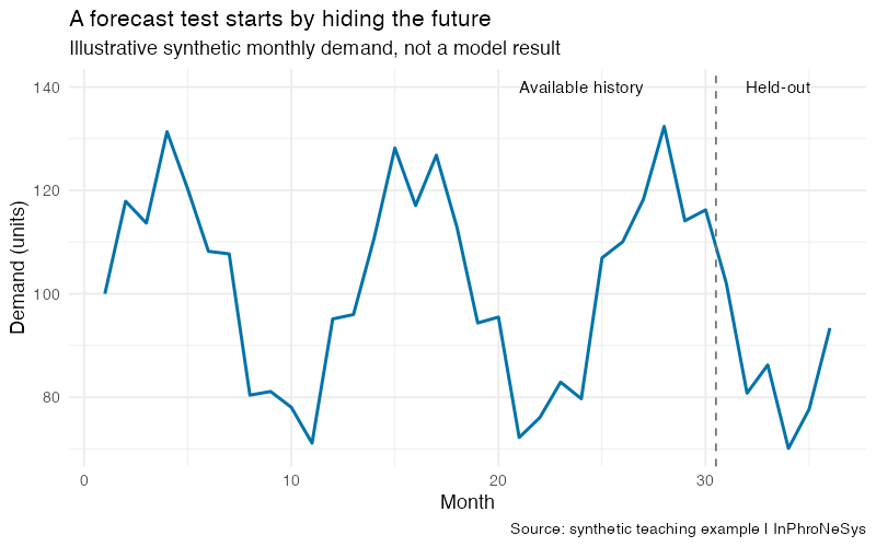
Choose a manageable set of products and the horizon that matters to your decisions. Include different demand patterns, including the awkward items, rather than selecting only smooth series that make every chart look respectable.
Compare the candidates with seasonal naive where appropriate, a suitable statistical method, and your current forecast. For intermittent demand, include a relevant intermittent-demand benchmark. Use several historical forecast origins and give every candidate only information available at the time.
Then examine more than the average error. Check bias, performance by product segment, uncertainty calibration, processing time, and the amount of planner intervention required. Keep a final untouched test period after selecting your model and settings.
The final question is operational: do the forecasts help you make better replenishment, inventory, or capacity decisions under realistic constraints?
That is the test I care about. A benchmark result can earn a model an invitation. Your planning process decides whether it gets a job.
Explore the model comparison
The companion dashboard shows the top ten reported entries for each of three selected metrics in Mistral’s technical-report comparison. Timestral’s larger checkpoints lead those views. You can also see how t0-gamma, TiRex-2, and international competitors compare.
This is a dated comparison from one published source, not a live ranking of every forecasting system. The wider GIFT-Eval board includes agents and other systems and can show a different order. The dashboard states its source, dates, metrics, and checkpoint differences.
Interactive Dashboard
Explore the data yourself. Adjust the parameters and watch the results update in real time.
European teams have earned a place on the shortlist. If you are responsible for demand planning, choose a few representative series, run a fair comparison, and keep the results. When the next model arrives, you will have something more useful than an opinion to compare it with.
Model details and sources checked 1 November 2026. Benchmark scores are publisher-reported; no new model evaluation was conducted for this article. The chart is a synthetic teaching illustration.
Show R code for the illustrative chart
tryCatch(source("Scripts/theme_inphronesys.R"), error=function(e) {
  message("Shared theme font unavailable; using local sans font and brand blue.")
  iph_colors <<- list(blue="#0073aa")
  theme_inphronesys <<- function(...) ggplot2::theme_minimal(base_size=13)
})
library(ggplot2)
d <- data.frame(month=1:36, demand=100+25*sin(2*pi*(0:35)/12)+8*sin((0:35)*2.4))
p <- ggplot(d,aes(month,demand))+geom_line(color=iph_colors$blue,linewidth=1)+geom_vline(xintercept=30.5,linetype="dashed",color="grey45")+annotate("text",x=24,y=140,label="Available history",size=4)+annotate("text",x=33.5,y=140,label="Held-out",size=4)+labs(title="A forecast test starts by hiding the future",subtitle="Illustrative synthetic monthly demand, not a model result",x="Month",y="Demand (units)",caption="Source: synthetic teaching example | InPhroNeSys")+theme_inphronesys()
ggsave("https://inphronesys.com/wp-content/uploads/2026/11/tsfm_forecast_test.png",p,width=8,height=5,dpi=100,bg="white")
Created with AI assistance under human editorial control.
Leave a Reply