
Every demand planner is circling the same nervous question. Will an AI foundation model make my forecasting toolkit obsolete? The pitch is seductive: point the model at your history, get a forecast, fire nobody, tune nothing. So I ran the race. For exactly €0, on my own laptop, I put one of Amazon’s forecasting AIs up against a pile of formulas older than the moon landing. 148 real retail series. Fair rules. One scoreboard.
The oldest formula on the grid dates to 1960. It won.
The setup: no home-field advantage
The data is real. I used aus_retail from the tsibbledata R package: 148 monthly retail-turnover series published by the Australian Bureau of Statistics, one for each State by Industry combination. Turnover is measured in Australian dollars, millions. The series are long. Depending on when each one starts, the training history runs from 345 to 417 months, ending in December 2016. Then every model forecasts the same 24 months, January 2017 through December 2018, and gets scored the same way.
Seven contenders lined up:
- Seasonal naive: repeat last year’s same-month value. The baseline everyone should have to beat.
- Naive: repeat last month’s value. Included mostly so we have a floor to laugh at.
- ETS (Holt-Winters): exponential smoothing with trend and seasonality. Born 1960.
- ARIMA: the other classical workhorse, fitted automatically.
- ETS + ARIMA combo: the simple average of the two point forecasts.
- Chronos-Bolt small: Amazon’s forecasting foundation model, 48 million parameters.
- Chronos-Bolt base: the bigger sibling, 205 million parameters.
The five classical models trained on each series. The two AIs did not. That word matters, so here it is in plain English.
Zero-shot means the AI never saw this data and never got tuned for it. Chronos-Bolt was pre-trained on a huge corpus of other time series, then asked to forecast retail turnover it had never met. No fitting. No parameter search. No covariates. You hand it the history, it hands you a forecast. That is the whole selling point: skip the modeling work entirely.
To keep the race honest, every forecast went through one scoring function. No model got a friendlier code path than any other.
One number to rank them all: MASE
I scored everything with MASE, the Mean Absolute Scaled Error (Hyndman & Koehler, 2006). It sounds fancy. It isn’t.
MASE compares each model’s error to a dead-simple benchmark: repeating last year’s seasonal pattern. A MASE of 1.0 means "as accurate as that free baseline." Below 1.0 beats the baseline. Above 1.0 loses to it. So 1.24 means "24% worse errors than just copying last year." The scale is the same across every series, which is why you can average it over 148 of them without the biggest series drowning out the rest. That’s the whole idea. One honest yardstick.
The scoreboard
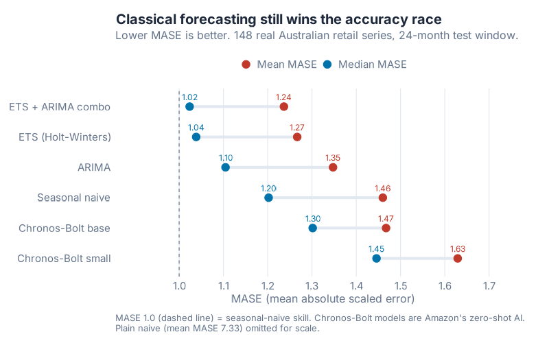
Here is the full leaderboard, ranked by mean MASE across all 148 series. Lower is better.
| Model | Family | Mean MASE | Median MASE | Mean RMSSE |
|---|---|---|---|---|
| ETS + ARIMA combo | Classical | 1.24 | 1.02 | 1.05 |
| ETS (Holt-Winters) | Classical | 1.27 | 1.04 | 1.09 |
| ARIMA | Classical | 1.35 | 1.10 | 1.14 |
| Seasonal naive | Classical | 1.46 | 1.20 | 1.26 |
| Chronos-Bolt base | AI foundation | 1.47 | 1.30 | 1.26 |
| Chronos-Bolt small | AI foundation | 1.63 | 1.45 | 1.38 |
| Naive | Classical | 7.33 | 5.09 | 5.73 |
Read the top and the middle of that table together. The classical ETS + ARIMA combination lands at 1.24. The best AI model, Chronos-Bolt base, lands at 1.47. That gap is 16% on mean error. ETS on its own, that 1960 formula, comes in at 1.27 and beats the AI by 14%. Call it 14 to 16% either way you slice it. The 66-year-old idea out-forecast the 205-million-parameter model, and it wasn’t close.
Now look one row up from the AI. Seasonal naive, the free baseline, scored 1.46. Chronos-Bolt base scored 1.47. On mean MASE that is a dead heat, and on RMSSE they tie exactly at 1.26. Amazon’s foundation model, zero-shot, matched the cheapest benchmark in forecasting. It did not beat it.
I’ll be blunt about what that means. Out of the box, on this data, the AI bought you baseline accuracy. Nothing more.
(And the plain naive model at 7.33? That’s what happens when you ignore seasonality in seasonal data. Leave it on the field as a reminder.)
One table row can flatter or bury a model, so here’s the whole spread. Each dot is one of the 148 series; the diamond marks each model’s median.
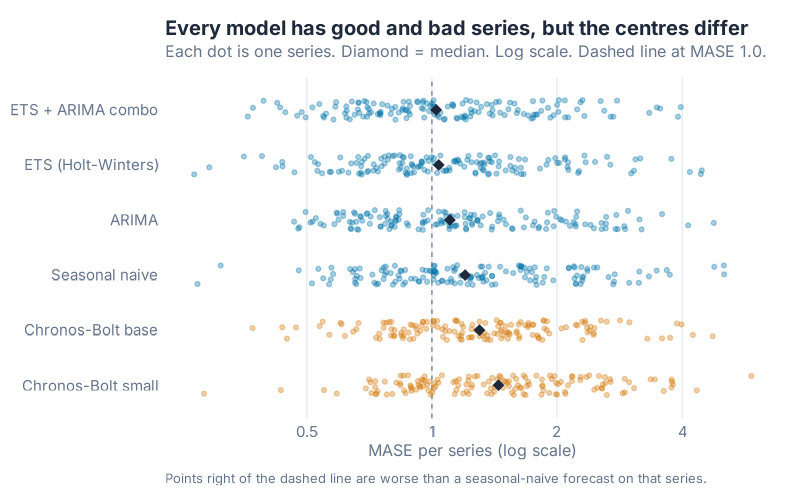
What jumped out at me is that every model has a long tail of ugly series stretching right past MASE 4.0. Nobody is safe everywhere. The difference is where the center of each cloud sits, and the classical diamonds sit visibly to the left of the two AI models. Same failure modes, better middle.
Two different ways to be "best"
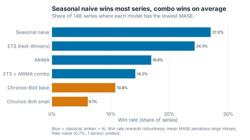
Averages hide things. So I also counted wins: on how many of the 148 series did each model post the single lowest MASE? The picture shifts.
| Model | Series won | Win rate |
|---|---|---|
| Seasonal naive | 40 | 27.0% |
| ETS (Holt-Winters) | 36 | 24.3% |
| ARIMA | 25 | 16.9% |
| ETS + ARIMA combo | 21 | 14.2% |
| Chronos-Bolt base | 16 | 10.8% |
| Chronos-Bolt small | 9 | 6.1% |
| Naive | 1 | 0.7% |
Wait. The combo had the best average but wins the fewest series of the serious contenders? Both facts are true, and they don’t fight. The combo wins on average because it rarely blows up. It has no catastrophic misses, so its mean stays low. Seasonal naive wins the most series because on smooth, strongly seasonal turnover it is genuinely hard to beat, series by series. One model avoids disasters. The other nails the easy cases. Different kinds of good.
Chronos-Bolt base won 16 series outright. Real, not zero. On the right series the AI is the best tool on the field. It just isn’t the best tool often enough to top a tuned classical model.
The horizon plot twist
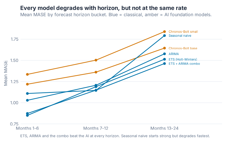
Forecast error grows as you look further out. But not at the same rate for everyone.
| Model | Months 1-6 | Months 7-12 | Months 13-24 |
|---|---|---|---|
| ETS + ARIMA combo | 0.87 | 1.15 | 1.46 |
| ETS (Holt-Winters) | 0.85 | 1.19 | 1.51 |
| ARIMA | 1.03 | 1.21 | 1.58 |
| Seasonal naive | 1.11 | 1.15 | 1.79 |
| Chronos-Bolt base | 1.22 | 1.36 | 1.64 |
| Chronos-Bolt small | 1.33 | 1.50 | 1.84 |
The trained classical models (ETS, ARIMA, combo) beat both AIs in every single bucket. No horizon rescues the foundation model against a fitted competitor. But watch the baseline. Seasonal naive is the best short-horizon model in the whole race at months 1 to 6 (1.11), then falls apart fastest. By the 13-to-24-month bucket it sits at 1.79, worse than Chronos-Bolt base at 1.64. Here’s the honest nuance: the AI overtakes the free baseline on long horizons, because copying last year drifts badly when a series trends. It still never overtakes a trained model. Repeating last year ages like milk. The AI ages a little better. The fitted models age best of all.
So what does the AI actually buy you?
Not accuracy. Speed.
Each Chronos model forecast all 148 series in under five seconds, zero-shot, with no fitting. The ETS + ARIMA combination took roughly 140 seconds to fit and forecast the same set on the same laptop. That’s more than 25 times slower for the classical winner. Configuration time? The AI needs none. You don’t choose a seasonal period, you don’t pick trend damping, you don’t stare at ACF plots. You send history, you get numbers.
That trade has a real shape. For a fleet of thousands of low-value SKUs where nobody will ever tune a model by hand, "baseline accuracy in seconds with zero setup" can be exactly the deal you want. Good enough, instant, free of babysitting. For a handful of high-value planning series that drive your S&OP numbers, where one point of accuracy moves real money, spending 140 seconds to fit a model that’s 14 to 16% better is the easiest trade in the building.
Scale did help the AI, for what it’s worth. Chronos-Bolt base beat Chronos-Bolt small by 11%. The bigger model is the better model. The foundation-model scaling story is visible in the numbers. It just wasn’t enough scaling to overtake a formula from 1960.
One series, up close
Averages are abstract. Look at a single series to see how these models actually behave.
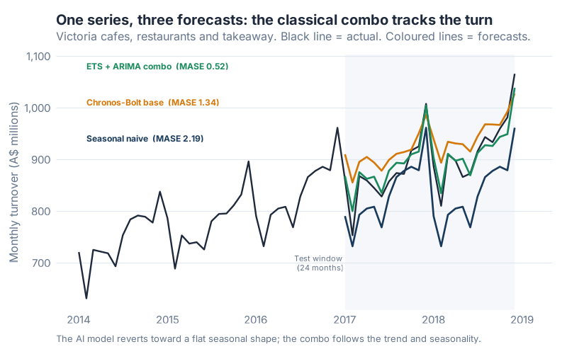
This is Victoria’s cafes, restaurants and takeaway food services: turnover climbing from about A$700M to A$1,050M a month, with a strong seasonal wave riding on a clear upward trend. Three forecasts, three personalities.
The ETS + ARIMA combo (MASE 0.52) reads the trend and the seasonality and rides both. Chronos-Bolt base (1.34) catches the seasonal shape but flattens the trend, reverting toward a level that the real series has already left behind. Seasonal naive (2.19) just stamps last year’s pattern onto a rising series and undershoots for two straight years. This one series is a clean illustration of the whole race, though I’ll caution it’s illustrative, not representative. On smoother, flatter series the ranking can invert. That’s what the win-rate table was telling you.
Where this breaks
I ran one race on one track. Before you carve the result into your vendor-selection deck, here is what this test does not prove.
- One dataset family. Australian retail turnover is monthly, strongly seasonal, and mostly trending. Intermittent demand, promotion-driven SKUs, short series, and high-frequency data could all tell a different story.
- One split, one regime. A single fixed test window (2017-2018), no rolling-origin evaluation. One pre-COVID economic period.
- Point forecasts only. I compared point forecasts (the fable mean against the Chronos median) and never scored the probability distributions. Chronos natively outputs quantiles, and I didn’t use that strength at all.
- Zero-shot by design. Chronos got no fine-tuning and no covariates. That’s the intended "out of the box" test, but fine-tuning could move the result.
- Turnover, not unit demand. The target is aggregate dollars, not SKU-level units. The dynamics of unit demand differ.
- Two AI sizes only. I tested Chronos-Bolt small and base, not the whole zoo of foundation models (TimesFM, Moirai, TimeGPT).
One more piece of context, because someone will raise it. Didn’t machine learning crush statistics in the M5 competition? Yes. In M5, the best ML method beat the best statistical benchmark by 22.4% (Makridakis et al., 2022). But those winners were gradient-boosted trees trained on the competition data with covariates. My test is the opposite setup: zero-shot, no training, no covariates. The two results don’t conflict. Trained ML on your data can win. An untuned foundation model, pointed cold at your history, did not win here. Buy the right sentence, not the headline.
Interactive Dashboard
Explore all 148 series and every model’s forecast yourself. Filter by state and industry, switch models on and off, and watch the leaderboard and per-series errors update as you go.
Interactive Dashboard
Explore the data yourself — adjust parameters and see the results update in real time.
Your next steps
Skip the abstract advice. Here’s what to actually do this week.
- Run this exact race on 20 of your own SKUs. The R and Python code is at the bottom of this post. Swap in your history, keep the scoring function, and see where your data lands. Twenty series is an afternoon.
- Measure any forecasting AI against your own seasonal naive before you sign anything. If a vendor can’t beat "repeat last year" on your data, you’re paying for a baseline you already have for free.
- Put MASE on your S&OP scorecard. One scale-free number, comparable across every SKU. Stop arguing about MAPE on low-volume items.
- Split your catalog by value, then pick the tool per tier. Foundation model for the long tail of thousands of cheap SKUs where nobody will ever tune anything. Fitted ETS or ARIMA for the high-value series that move your plan.
- Score the distribution, not just the point, on your next test. Chronos outputs quantiles. If you care about safety stock and service levels, a point forecast is the wrong thing to be grading.
The foundation models are coming for the boring 80% of your catalog, and honestly, they can have it. The 20% that matters still belongs to a formula older than the pocket calculator. Race them yourself before you believe either of us.
Show R Code
This script fits the classical models, reads the Chronos forecasts, and scores all seven models through one identical MASE/RMSSE code path. It reads the train/test splits produced by Scripts/horserace/export_aus_retail.R (which exports the real aus_retail data from tsibbledata).
# =============================================================================
# score_horserace.R — Forecasting horse race scoring (single code path)
# =============================================================================
# Fits classical models on the aus_retail train split, reads the Chronos
# foundation-model forecasts, and scores EVERY model through ONE MASE/RMSSE
# function so no model gets an unfair code path.
#
#   Classical (fable): SNAIVE, NAIVE, ETS (auto), ARIMA (auto), ETS+ARIMA combo
#   Foundation (read): amazon/chronos-bolt-small, amazon/chronos-bolt-base
#
# Scoring (Hyndman & Koehler 2006, seasonal m = 12):
#   scale (MASE denom) = mean_{t=m+1..n} |Y_t - Y_{t-m}|   on TRAIN
#   MASE  = mean_{h}|actual_h - fcast_h| / scale
#   RMSSE = sqrt(mean_{h}(actual_h - fcast_h)^2) / sqrt(mean_{t}(Y_t-Y_{t-m})^2)
#
# Run from project root:
#   Rscript Scripts/horserace/score_horserace.R
# =============================================================================

suppressPackageStartupMessages({
  library(fpp3)
  library(dplyr)
  library(tidyr)
  library(readr)
  library(jsonlite)
})

set.seed(42)

res_dir <- "Research/horserace_results"
M       <- 12L   # seasonal period (monthly)

# --- 1. Load data -----------------------------------------------------------
to_ym <- function(x) yearmonth(as.Date(paste0(x, "-01")))

train_raw <- read_csv(file.path(res_dir, "train.csv"), show_col_types = FALSE)
test_raw  <- read_csv(file.path(res_dir, "test.csv"),  show_col_types = FALSE)
chronos   <- read_csv(file.path(res_dir, "chronos_forecasts.csv"),
                      show_col_types = FALSE)

train_ts <- train_raw |>
  mutate(month = to_ym(month)) |>
  as_tsibble(index = month, key = series_id)

n_series <- n_distinct(train_ts$series_id)
cat(sprintf("Loaded %d series | train rows %d | test rows %d | chronos rows %d\n",
            n_series, nrow(train_raw), nrow(test_raw), nrow(chronos)))

# --- 2. Fit classical models (timed separately for the effort comparison) ---
fit_forecast <- function(formula_expr, label) {
  t <- system.time({
    mbl <- train_ts |> model(m = formula_expr)
    fc  <- mbl |> forecast(h = 24)
  })
  cat(sprintf("  %-8s fitted+forecast in %5.1f s\n", label, t[["elapsed"]]))
  list(
    forecast = fc |>
      as_tibble() |>
      transmute(series_id, month, model = label, forecast = .mean),
    seconds = unname(t[["elapsed"]])
  )
}

cat("Fitting classical models on train (through 2016-12), h = 24:\n")
snaive_r <- fit_forecast(SNAIVE(turnover ~ lag("year")), "snaive")
naive_r  <- fit_forecast(NAIVE(turnover),                 "naive")
ets_r    <- fit_forecast(ETS(turnover),                   "ets")
arima_r  <- fit_forecast(ARIMA(turnover),                 "arima")

# ETS + ARIMA average combination — point forecast is the mean of the two
# point forecasts, so we derive it directly (timing = ets + arima cost).
combo_fc <- ets_r$forecast |>
  rename(f_ets = forecast) |>
  inner_join(arima_r$forecast |> rename(f_arima = forecast),
             by = c("series_id", "month")) |>
  transmute(series_id, month, model = "ets_arima_combo",
            forecast = (f_ets + f_arima) / 2)
combo_seconds <- ets_r$seconds + arima_r$seconds
cat(sprintf("  %-8s derived from ets+arima (%5.1f s combined)\n",
            "combo", combo_seconds))

# --- 3. Build ONE long forecast table (fable + chronos) ---------------------
# Normalise everyone to (series_id, month=char "YYYY-MM", model, forecast).
fable_long <- bind_rows(
  snaive_r$forecast, naive_r$forecast, ets_r$forecast,
  arima_r$forecast, combo_fc
) |>
  mutate(month = format(as.Date(month), "%Y-%m"))

chronos_long <- chronos |>
  transmute(series_id, month = as.character(month), model, forecast)

all_fc <- bind_rows(fable_long, chronos_long)

stopifnot(!anyNA(all_fc$forecast))
cat(sprintf("Combined forecast table: %d rows, %d models, %d series\n",
            nrow(all_fc), n_distinct(all_fc$model), n_distinct(all_fc$series_id)))

# --- 4. Per-series scale factors from TRAIN (seasonal naive, m = 12) --------
scales_tbl <- train_raw |>
  arrange(series_id, month) |>
  group_by(series_id) |>
  summarise(
    mae_scale  = mean(abs(turnover - lag(turnover, M)),   na.rm = TRUE),
    rmse_scale = sqrt(mean((turnover - lag(turnover, M))^2, na.rm = TRUE)),
    .groups = "drop"
  )
stopifnot(all(scales_tbl$mae_scale > 0))

# --- 5. THE single scoring code path ----------------------------------------
# Join forecasts to test actuals + per-series scale, then every model is
# scored by exactly this pipeline. No branch is model-specific.
scored <- all_fc |>
  inner_join(test_raw, by = c("series_id", "month")) |>   # brings in turnover (actual)
  inner_join(scales_tbl, by = "series_id") |>
  rename(actual = turnover) |>
  arrange(series_id, model, month) |>
  group_by(series_id, model) |>
  mutate(h = row_number()) |>                              # horizon index 1..24
  ungroup()

# sanity: each (series, model) must have all 24 test points
per_pair <- scored |> count(series_id, model)
stopifnot(all(per_pair$n == 24))

mase_by_series <- scored |>
  group_by(series_id, model) |>
  summarise(
    mase  = mean(abs(actual - forecast)) / first(mae_scale),
    rmsse = sqrt(mean((actual - forecast)^2)) / first(rmse_scale),
    .groups = "drop"
  )

# horizon buckets: months 1-6, 7-12, 13-24
bucket_of <- function(h) dplyr::case_when(
  h <= 6  ~ "h01_06",
  h <= 12 ~ "h07_12",
  TRUE    ~ "h13_24"
)
mase_by_bucket <- scored |>
  mutate(bucket = bucket_of(h)) |>
  group_by(series_id, model, bucket) |>
  summarise(mase = mean(abs(actual - forecast)) / first(mae_scale),
            .groups = "drop")

# --- 6. Summaries -----------------------------------------------------------
summary_tbl <- mase_by_series |>
  group_by(model) |>
  summarise(
    mean_mase   = mean(mase),
    median_mase = median(mase),
    mean_rmsse  = mean(rmsse),
    .groups = "drop"
  ) |>
  arrange(mean_mase)

# win rate: per series, model(s) with the minimum MASE. Ties split evenly.
wins <- mase_by_series |>
  group_by(series_id) |>
  mutate(is_min = mase == min(mase),
         win_weight = is_min / sum(is_min)) |>
  ungroup()
n_ties <- wins |>
  group_by(series_id) |>
  summarise(tie = sum(is_min) > 1, .groups = "drop") |>
  summarise(n = sum(tie)) |> pull(n)
winrate_tbl <- wins |>
  group_by(model) |>
  summarise(win_rate = sum(win_weight) / n_series, .groups = "drop") |>
  arrange(desc(win_rate))

bucket_tbl <- mase_by_bucket |>
  group_by(model, bucket) |>
  summarise(mean_mase = mean(mase), .groups = "drop") |>
  pivot_wider(names_from = bucket, values_from = mean_mase) |>
  arrange(h01_06)

timing_tbl <- tibble(
  model   = c("snaive", "naive", "ets", "arima", "ets_arima_combo"),
  seconds = c(snaive_r$seconds, naive_r$seconds, ets_r$seconds,
              arima_r$seconds, combo_seconds)
)

# --- 7. Verification print --------------------------------------------------
cat("\n================ LEADERBOARD (mean MASE, ascending) ================\n")
print(as.data.frame(summary_tbl), digits = 4, row.names = FALSE)
cat("\n================ WIN RATE (share of 148 series) ====================\n")
print(as.data.frame(winrate_tbl |> mutate(win_rate = round(win_rate, 4))),
      row.names = FALSE)
cat(sprintf("Series with ties at the top: %d\n", n_ties))
cat("\n================ MASE BY HORIZON BUCKET ============================\n")
print(as.data.frame(bucket_tbl), digits = 4, row.names = FALSE)
cat("\n================ CLASSICAL FITTING WALL-CLOCK (s) =================\n")
print(as.data.frame(timing_tbl), digits = 3, row.names = FALSE)

# --- 8. Cross-check vs the team lead's rough Python numbers ------------------
rough <- tibble(
  model       = c("chronos_bolt_small", "chronos_bolt_base", "snaive"),
  rough_mean  = c(1.63, 1.47, 1.46),
  rough_median= c(1.45, 1.30, 1.20)
)
check <- summary_tbl |>
  inner_join(rough, by = "model") |>
  mutate(d_mean = round(mean_mase - rough_mean, 3),
         d_median = round(median_mase - rough_median, 3),
         flag = ifelse(abs(d_mean) > 0.02 | abs(d_median) > 0.02, "CHECK", "ok"))
cat("\n================ CROSS-CHECK vs rough Python sanity =================\n")
print(as.data.frame(check |>
  select(model, mean_mase, rough_mean, d_mean,
         median_mase, rough_median, d_median, flag)),
  digits = 4, row.names = FALSE)

# --- 9. Persist outputs -----------------------------------------------------
write_csv(mase_by_series |> arrange(series_id, model),
          file.path(res_dir, "mase_by_series.csv"))

# Full forecast table (fable + chronos) so the images script never refits.
write_csv(all_fc |> arrange(series_id, model, month),
          file.path(res_dir, "forecasts_all.csv"))

summary_out <- summary_tbl |>
  left_join(winrate_tbl, by = "model") |>
  left_join(bucket_tbl,  by = "model") |>
  left_join(timing_tbl,  by = "model")

json_out <- list(
  meta = list(
    n_series          = n_series,
    forecast_rows      = nrow(all_fc),
    rows_per_model     = nrow(all_fc) / n_distinct(all_fc$model),
    h                  = 24L,
    train_span         = paste(min(train_raw$month), max(train_raw$month), sep = " .. "),
    test_span          = paste(min(test_raw$month),  max(test_raw$month),  sep = " .. "),
    mase_definition    = "Hyndman & Koehler 2006, seasonal m=12; denom = in-sample MAE of 12-month seasonal naive on train",
    fable_point        = "mean (.mean, fable default)",
    chronos_point      = "median (q=0.5)",
    n_series_with_ties = n_ties
  ),
  models = summary_out |>
    transmute(model, mean_mase, median_mase, mean_rmsse, win_rate,
              mase_h01_06 = h01_06, mase_h07_12 = h07_12, mase_h13_24 = h13_24,
              fit_seconds = seconds) |>
    purrr::transpose(),
  cross_check = check |>
    select(model, mean_mase, rough_mean, d_mean,
           median_mase, rough_median, d_median, flag) |>
    purrr::transpose()
)
write_json(json_out, file.path(res_dir, "scores_summary.json"),
           pretty = TRUE, auto_unbox = TRUE, digits = 6)

cat(sprintf("\nWrote %s (%d rows)\n",
            file.path(res_dir, "mase_by_series.csv"), nrow(mase_by_series)))
cat(sprintf("Wrote %s\n", file.path(res_dir, "scores_summary.json")))
cat("Done.\n")
Show Python Code (Chronos)
House rule: Python is welcome when the subject library is Python-native, and this post is the poster child. Chronos-Bolt ships as a Python package, so the zero-shot forecasts live here. Point forecast is the median (the 0.5 quantile).
#!/usr/bin/env python3
"""
Zero-shot Chronos-Bolt forecasts for the horse race.

Reads Research/horserace_results/train.csv (148 aus_retail series through
2016-12), forecasts h=24 months (2017-01..2018-12) with amazon/chronos-bolt-small
and amazon/chronos-bolt-base, entirely zero-shot (no fine-tuning, no covariates).
Point forecast = median (0.5 quantile). Writes chronos_forecasts.csv and
timing_chronos.json. Run from project root.
"""

import json
import time
from pathlib import Path

import pandas as pd
import torch
from chronos import BaseChronosPipeline

H = 24
OUT = Path("Research/horserace_results")
MODELS = {
    "chronos_bolt_small": "amazon/chronos-bolt-small",
    "chronos_bolt_base": "amazon/chronos-bolt-base",
}

device = "mps" if torch.backends.mps.is_available() else "cpu"
print(f"device: {device}")

train = pd.read_csv(OUT / "train.csv")
series_ids = sorted(train["series_id"].unique())
print(f"series: {len(series_ids)}, train rows: {len(train)}")

contexts = []
for sid in series_ids:
    vals = train.loc[train["series_id"] == sid].sort_values("month")["turnover"].to_numpy()
    contexts.append(torch.tensor(vals, dtype=torch.float32))

months = pd.period_range("2017-01", periods=H, freq="M").strftime("%Y-%m").tolist()

rows = []
timing = {}
for model_key, model_name in MODELS.items():
    pipeline = BaseChronosPipeline.from_pretrained(model_name, device_map=device,
                                                   torch_dtype=torch.float32)
    t0 = time.time()
    quantiles, _ = pipeline.predict_quantiles(inputs=contexts, prediction_length=H,
                                              quantile_levels=[0.5])
    elapsed = time.time() - t0
    timing[model_key] = {"model": model_name, "seconds_forecast": round(elapsed, 2),
                         "device": device, "n_series": len(series_ids), "h": H}
    print(f"{model_key}: {elapsed:.1f}s for {len(series_ids)} series")
    med = quantiles[:, :, 0]  # (n_series, H)
    for i, sid in enumerate(series_ids):
        for j, m in enumerate(months):
            rows.append({"series_id": sid, "month": m, "model": model_key,
                         "forecast": float(med[i, j])})

pd.DataFrame(rows).to_csv(OUT / "chronos_forecasts.csv", index=False)
(OUT / "timing_chronos.json").write_text(json.dumps(timing, indent=2))
print(f"wrote {OUT/'chronos_forecasts.csv'} ({len(rows)} rows) and timing_chronos.json")
References
- Ansari, A. F., Stella, L., Turkmen, C., Zhang, X., Mercado, P., Shen, H., Shchur, O., Rangapuram, S. S., Pineda Arango, S., Kapoor, S., Zschiegner, J., Maddix, D. C., Wang, H., Mahoney, M. W., Torkkola, K., Wilson, A. G., Bohlke-Schneider, M., & Wang, Y. (2024). Chronos: Learning the Language of Time Series. arXiv:2403.07815. https://arxiv.org/abs/2403.07815. Chronos-Bolt is Amazon’s faster T5-based variant; model cards at chronos-bolt-base (205M params) and chronos-bolt-small (48M params).
- Winters, P. R. (1960). Forecasting Sales by Exponentially Weighted Moving Averages. Management Science, 6(3), 324-342. https://doi.org/10.1287/mnsc.6.3.324. The seasonal Holt-Winters method: 2026 minus 1960 is the 66 years in the title.
- Holt, C. C. (1957/2004). Forecasting seasonals and trends by exponentially weighted moving averages. International Journal of Forecasting, 20(1), 5-10. https://doi.org/10.1016/j.ijforecast.2003.09.015.
- Hyndman, R. J., & Koehler, A. B. (2006). Another look at measures of forecast accuracy. International Journal of Forecasting, 22(4), 679-688. https://doi.org/10.1016/j.ijforecast.2006.03.001. The MASE metric.
- Australian Bureau of Statistics retail turnover, monthly, distributed as
aus_retailin thetsibbledataR package. https://tsibbledata.tidyverts.org/. - Makridakis, S., Spiliotis, E., & Assimakopoulos, V. (2022). M5 accuracy competition: Results, findings, and conclusions. International Journal of Forecasting, 38(4), 1346-1364. https://doi.org/10.1016/j.ijforecast.2021.11.013.
Leave a Reply