
The 20% ask that the indices priced at 2%
A supplier asked for 20.4% on a machined metal part. Nothing about that is obviously absurd. Metal was up, wages were up, and every letter in the folder said the same thing.
What the published indices actually support is 2.3%.
Here is the split. Take the ask apart across that part’s own cost structure and escalate each bucket with the index that drives it. Material is 35.5% of the price, and the Eurostat producer price index for basic metals moved 5.5% over the window since this pair’s previous price change. Labour is 31.0% and plant burden another 20.1%, both escalated on the labour cost index, which moved 0.7%. The remaining 13.5% is SG&A and profit, carried as a percentage of price, so it inflates automatically and needs no help.
That leaves 18.1% with no index behind it, and on the trailing twelve months of spend for that one part and supplier, 18.1% is worth EUR 11,288. Across the whole file, six flagged increases carry EUR 43,017 of unexplained ask.
That is not money in the bank. It’s a number you can put on the table and make somebody explain. Which is a different and more useful thing.
The rest of this post is how it works, where it’s right, and where it isn’t. Four questions, four lenses, one R script you point at your own PO export. It also gets three things wrong. Those turned out to be the most interesting part.
What the workbench is, and where it came from
Scripts/price_anomaly_workbench.R reads a purchase-order export and answers four questions that buyers actually ask. The engine isn’t mine. It’s Rob Hyndman’s weird package (version 3.0.0), which he presented in Ihaka Lecture 2026 #3, "Spotting the Weird Ones" at the University of Auckland on 6 August 2026, the day before this post went up. The "four kinds of weird" framing is mine, not his, so don’t go looking for it in the lecture.
The idea I stole is the conditional fit below. Hyndman demonstrates it on wine: fit lm(log(price) ~ points) and the residuals surface bottles that are overpriced for their quality score, which is a much sharper question than "which bottles are expensive." Swap quality points for order quantity and you have a purchasing tool.
| Lens | The buyer’s question | What it does |
|---|---|---|
| 1 | Which lines are weird at all? | Kernel density over (log quantity, log price), within part family |
| 2 | What discount curve did I actually get? | Fits price given quantity and part, then scores what the model can’t explain |
| 3 | Who hides margin where? | Scores each supplier’s cost breakdown against its peers in the same family |
| 4 | Was that increase justified? | Index attribution, pass-through asymmetry, peer benchmark, threshold bunching |
The demo data is a synthetic PO history: 3,505 lines, 40 parts in 4 families, 10 invented suppliers, 91 part by supplier pairs, EUR 10,921,658 of spend from 2023-01-01 to 2026-06-28, with 45 anomalies of 7 types planted so recall can be measured instead of asserted. The supplier data is fabricated. The indices it moves against are real Eurostat series, pulled 2026-08-07.
One install note that will save you an hour. On macOS, run brew install --cask xquartz before you install weird. The package needs aplpack, whose NAMESPACE imports tcltk even though its DESCRIPTION only lists it under Suggests, and tcltk on macOS links against X11. Without XQuartz the install dies at the lazy-load step with an error that points nowhere near the actual cause. Ask me how I know.
The whole argument is conditioning
Here’s the claim I’ll defend for the rest of the post. Point a general anomaly detector at a raw price column and it will spend your attention on prices that are exactly correct. That’s worse than finding nothing, because finding nothing at least costs you nothing.
The demo data is built to prove it. Sixteen lines are genuinely mispriced. Eight more are decoys: freak order quantities priced precisely on the contractual discount curve. A decoy is a one-off tiny order at the correct one-off tiny-order price. There is nothing wrong with it. Decoys exist to measure wasted attention.
The density view is the honest baseline, and it’s what most people mean by anomaly detection. Two-dimensional density over log quantity and log price. Nothing more.
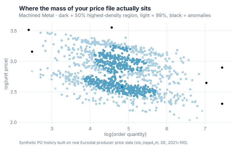
That view is not useless. It’s just answering a question nobody asked. Everything on the outside edge is unusual, and being unusual is not the same as being wrong.
Now the head-to-head, at the same threshold, over all 3,505 lines:
| Method | Flags | Real problems caught | Decoys flagged | Precision |
|---|---|---|---|---|
| Lens 1: density on (quantity, price) | 46 | 7/16 | 8/8 | 15% |
| Lens 2: given quantity | 35 | 6/16 | 0/8 | 17% |
| Lens 2: given quantity and part | 36 | 16/16 | 0/8 | 44% |
Read the decoy column first. The unconditional detector flagged every single decoy. All eight. It could not tell the difference between "this price is wrong" and "this quantity is unusual," because it has no concept of a price being appropriate for anything.
Then read the recall column. Conditioning on quantity alone barely helps, and actually loses one real problem. Add part identity and recall goes from 7/16 to 16/16 while the flag count falls from 46 to 36. Fewer alerts, every planted problem caught, zero decoys. My read is that this single modelling choice matters more than any threshold you will ever tune, and it’s the one most anomaly-detection write-ups skip entirely.
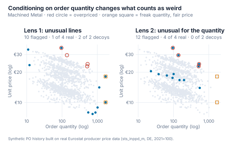
The chart shows one family rather than all four, so its counts are smaller than the headline table: within Machined Metal, the density view raises 10 flags, catching 1 of 4 real problems and both decoys. the conditional fit raises 12, catching 4 of 4 and neither decoy. What jumped out at me is that the two methods barely overlap. Across the full file, only 7 lines are flagged by both. They are looking at different things, and the density view’s question is not the one a buyer needs answered.
On threshold choice, since somebody will ask:
| Threshold | Lens 1 | Lens 2 (quantity) | Lens 2 (quantity and part) |
|---|---|---|---|
| 0.05 | 190 flags, 11/16, 8/8 decoys | 175 flags, 11/16, 0/8 | 173 flags, 16/16, 0/8 |
| 0.01 | 46 flags, 7/16, 8/8 | 35 flags, 6/16, 0/8 | 36 flags, 16/16, 0/8 |
| 0.001 | 17 flags, 6/16, 7/8 | 4 flags, 4/16, 0/8 | 8 flags, 8/16, 0/8 |
Start at 0.01. At 0.05 the tool hands you 173 flags on a 3,505-line file and no buyer alive will read them. At 0.001 you lose half the real problems to look tidy.
The discount curve you actually received
The conditional fit has a second output that is arguably more useful than the flags, and it costs nothing extra. The fitted slope of log price on log quantity is your empirical volume-discount elasticity. Not the one in the contract. The one you got.
| Family | Contracted | Fitted (part effects) | Fitted (naive pooled) | Discount per doubling |
|---|---|---|---|---|
| Injection Moulded Plastics | −0.180 | −0.177 | −0.184 | −11.5% |
| Machined Metal | −0.120 | −0.118 | −0.113 | −7.9% |
| PCB Assemblies | −0.220 | −0.217 | −0.215 | −13.9% |
| Cable Harnesses | −0.150 | −0.145 | −0.117 | −9.6% |
Convert the elasticity to something you can say out loud with 2^elasticity − 1. For plastics: 2^(−0.1767) − 1 = 0.8847 − 1 = −11.5%. Double the order, drop the unit price 11.5%.
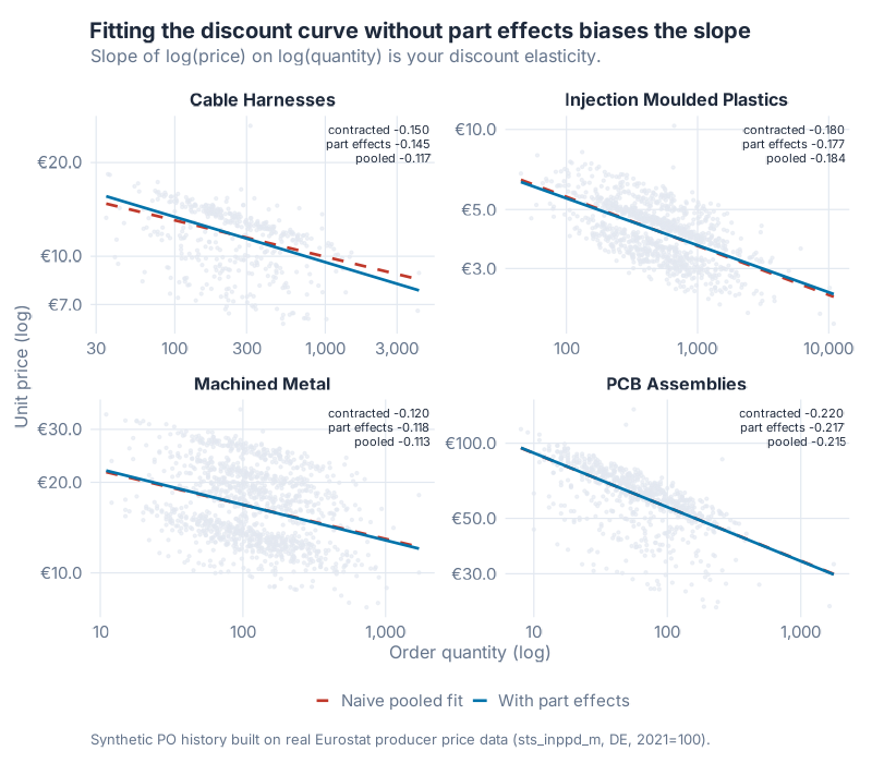
Look at Cable Harnesses. The naive pooled fit reads −0.117 against a contracted −0.150, understating the discount you’re owed by 0.033 of elasticity. Part effects fix it. Mean absolute error across the four families is 0.0032 with part effects against 0.0121 without, and residual standard deviation falls 72% on average (Machined Metal, 0.2772 to 0.0609). The other three families survive the naive fit intact, so treat this as one family’s warning rather than a rule. It’s enough of a warning.
Two earlier posts cover the contract side of elasticity properly, so I won’t re-teach it here: Quantity Discount Analysis on the trap in published discount schedules, and Your Supplier Isn’t Offering a Discount on what a price break is worth once you carry the inventory.
Who hides margin where
The cost-structure check takes the cost breakdowns your suppliers submitted and asks which ones sit oddly against their own peer group. One technical note, because it bit us: a four-bucket breakdown sums to one, so it lives on a simplex with three free dimensions. Collapse to material, labour, and overhead-plus-margin, then score two of the three. Score all three and you’ve fed the detector a perfectly collinear column.
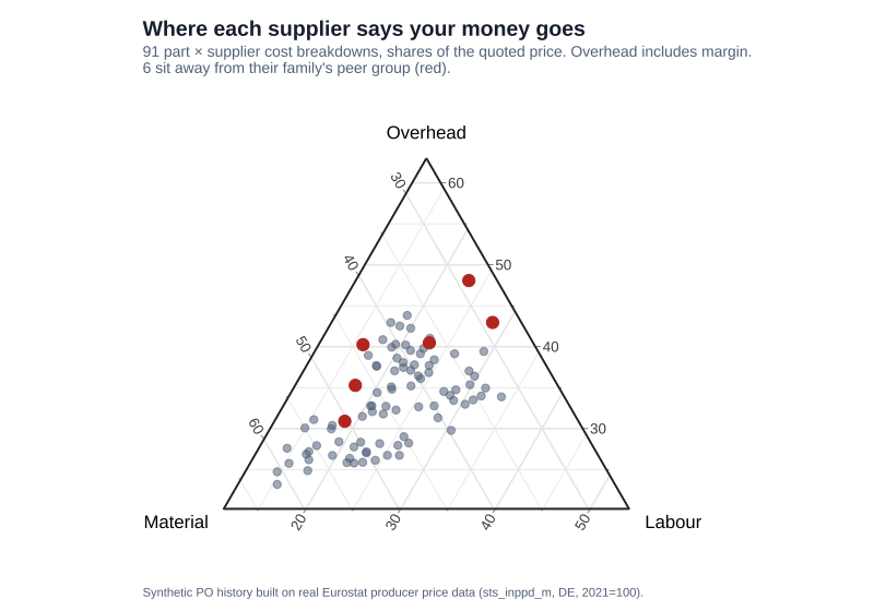
Of 91 breakdowns, 4 had margin quietly shifted out of material and into SG&A. The lens flagged 6. It caught all 4, with 2 false positives.
| Part | Supplier | Planted | Material | Labour | Overhead + margin | p |
|---|---|---|---|---|---|---|
| CAB-107 | Dornbach Kabeltechnik | yes | 0.367 | 0.229 | 0.405 | 0.0000 |
| PLA-184 | Nordhalle Kunststoff | yes | 0.287 | 0.232 | 0.481 | 0.0000 |
| PCB-107 | Ravensfeld Elektronik | yes | 0.438 | 0.160 | 0.402 | 0.0000 |
| MET-149 | Ostheim Praezision | yes | 0.287 | 0.283 | 0.430 | 0.000068 |
| PLA-121 | Vellmar Polymer | no | 0.471 | 0.177 | 0.353 | 0.00012 |
| CAB-114 | Aschenfeld Leitungen | no | 0.504 | 0.187 | 0.309 | 0.0045 |
Two false positives out of six is a fine trade when the output is six questions to ask, not six accusations to make.
The function that should have worked, and didn’t
Before the escalation check can ask whether an increase was justified, it has to find the increases. weird ships an obvious candidate: hampel_anomalies(), which compares each point to a rolling median and flags anything more than k scaled MADs away.
It caught nothing. Zero out of five.
| Method | Flags | Caught | Recall |
|---|---|---|---|
hampel_anomalies() on price levels |
10 | 0 | 0/5 |
hampel_anomalies() on first differences |
16 | 2 | 2/5 |
surprisals_prob() on first differences |
4 | 2 | 2/5 |
The reason is structural, and once you see it you can’t unsee it. Hampel detects spikes. A price increase is a step. The rolling median climbs the step along with the series, the deviation stays small, and nothing fires. The function is working exactly as designed on data it was never designed for.
Differencing the series first turns the step into a spike, and then it works. Better still, score the differences with surprisal probabilities instead: same recall, 4 flags instead of 16, and it returns a probability you can rank rather than a yes-or-no verdict at a threshold you guessed. That last move is Hyndman’s own advice from the lecture, applied to a function in his own package that shipped with a threshold.
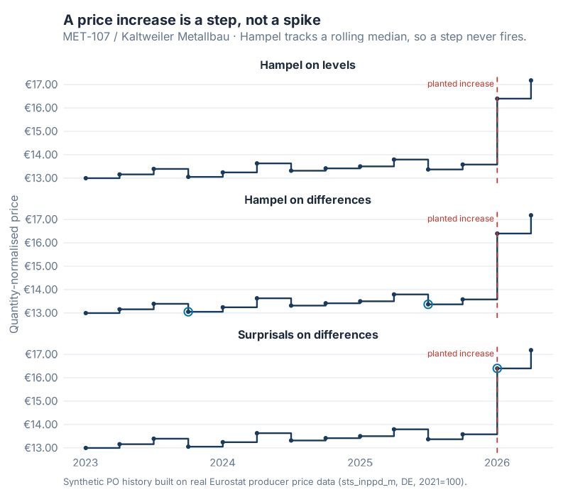
The top panel of that chart is empty on purpose. I left it in because a blank panel makes the point better than a paragraph does.
The number you take into the meeting
Now the attribution. For each flagged increase, split the ask across that pair’s cost buckets and escalate each one:
justified % = material share × Δ material index + labour share × Δ labour index + burden share × Δ labour index + SG&A share × 0
Then unexplained % = ask % − justified %. The window runs from that pair’s previous actual price change, because that’s the interval the supplier is implicitly claiming inflation over.
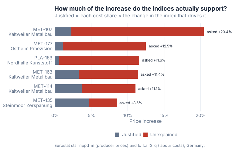
Worked, for the opening example. MET-107 with Kaltweiler Metallbau, 2026-Q1, window 2025-10-01 to 2026-01-01:
material : 0.3552 × +5.4735% = +1.9441%
labour   : 0.3098 × +0.6838% = +0.2118%
burden   : 0.2005 × +0.6838% = +0.1371%
sga      : 0.1345 ×  0.0000% = +0.0000%
justified                    = +2.2930%
ask                          = +20.4419%
unexplained                  = +18.1489%
Index attribution flagged seven asks. Only six carry money, and the seventh is the one I’d point to if somebody accuses this tool of being built to hunt villains. PCB-156 with Ravensfeld Elektronik, 2024-Q1: the ask was −2.95% and the indices justified only −0.42%. They cut their price by more than they had to, leaving 2.53% unexplained in the buyer’s favour. Same test, opposite sign.
Multiply each unexplained percentage by the trailing twelve months of spend on that pair and you have a euro figure per line item. One definition point, because it changes what the number means. That window is a fixed twelve months from the end of the file, not a window measured from each increase. A buyer is asking what the ask will cost going forward, and last year’s volume is the best available proxy for next year’s. It is not a bill for what the increase has already cost you.
For the six increases:
| Part | Supplier | Unexplained | 12m spend | EUR at stake |
|---|---|---|---|---|
| PLA-163 | Nordhalle Kunststoff | +11.05% | 148,095 | 16,365 |
| MET-177 | Ostheim Praezision | +11.38% | 130,090 | 14,805 |
| MET-107 | Kaltweiler Metallbau | +18.15% | 62,197 | 11,288 |
| MET-163 | Kaltweiler Metallbau | +8.11% | 3,189 | 259 |
| MET-114 | Kaltweiler Metallbau | +7.36% | 3,218 | 237 |
| MET-135 | Steinmoor Zerspanung | +3.82% | 1,677 | 64 |
| TOTAL | EUR 43,017 |
Total unexplained ask across the six flagged increases: EUR 43,017. (The script totals unrounded values, so the rounded column won’t reconcile to the last euro. Quote the total, not the arithmetic.)
Against EUR 10,921,658 of total spend that’s 0.39%, computed over three and a half years rather than one. Two things about that figure. It is a negotiating position, not a saving: it’s the size of the gap between what was asked and what published indices support, and it becomes real money only if somebody wins an argument. And the top three rows carry 98.7% of it, which is the usual shape. Three conversations get you almost all of the value.
The ratchet: pass-through that only works one way
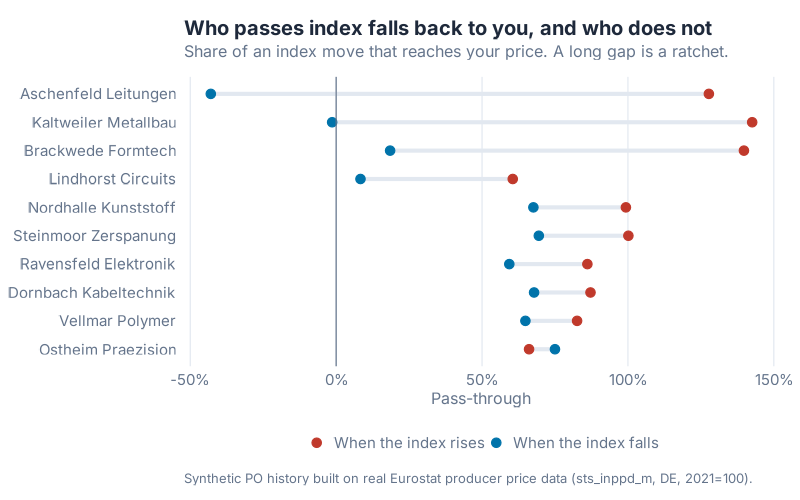
The ratchet test asks a question nobody’s price file answers directly. When the index goes up, does your supplier pass it on? And when it goes down, do they pass that on too?
Regress each announced ask on the index move since that supplier’s previous change, splitting the move into its positive and negative parts. Two coefficients per supplier. The gap between them is the ratchet.
| Supplier | β up | β down | Asymmetry | R² |
|---|---|---|---|---|
| Aschenfeld Leitungen | 1.277 | −0.430 | 1.707 | 0.81 |
| Kaltweiler Metallbau | 1.426 | −0.014 | 1.440 | 0.86 |
| Brackwede Formtech | 1.398 | 0.185 | 1.213 | 0.82 |
| Lindhorst Circuits | 0.605 | 0.083 | 0.522 | 0.44 |
| Nordhalle Kunststoff | 0.993 | 0.676 | 0.317 | 0.20 |
| Ostheim Praezision (10th of 10) | 0.661 | 0.750 | −0.089 | 0.64 |
Six of the ten suppliers are shown: the top five by asymmetry, plus the bottom-ranked one for contrast. Four suppliers were built to ratchet. All four came back in the top four positions, with a clean gap of 0.205 between fourth place (0.522) and fifth (0.317). Aschenfeld’s β down of −0.430 is the one to stare at: when their input index fell, their prices went up.
One trap, because I fell into it. Run this regression on period-by-period data instead of on change events and it returns nonsense, in our case per-supplier coefficients swinging from roughly minus 300% to plus 300%. Prices move at six- or twelve-month reviews while the index moves monthly, so period-by-period you are mostly regressing zeros on non-zeros. Measure the index move over the window between actual changes, or don’t measure it.
The most expensive pattern in the file is not an anomaly
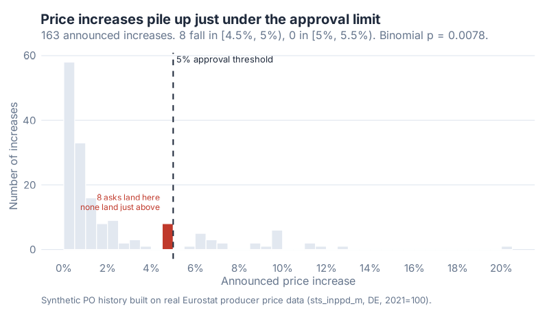
Your approval limit is 5%. Anything at or above it goes to your manager. Here is the distribution of announced increases:
| Bin | Count |
|---|---|
| [4.5%, 5.0%), just below the limit | 8 |
| [5.0%, 5.5%), just above | 0 |
Eight asks parked in the half-point below the limit. None in the half-point above. Under any smooth distribution those two adjacent bins should look similar; a binomial test on 8 versus 0 gives p = 0.0078. All eight were planted, and they came from 2 of the 10 suppliers, who do it as policy.
Now the part that matters. The per-increase detector caught zero of the eight. Not because it’s badly tuned. Because a 4.7% ask is engineered to look ordinary, and it succeeds. No detector scoring one increase at a time will ever flag it, since individually there is nothing to flag. The pattern exists only in the shape of the distribution.
The most expensive thing in a price file is often not an outlier at all. It’s a habit. And habits are invisible one row at a time.
Where this breaks
Six honest limitations. This section is longer than I’d like, which is usually a sign it’s the true one.
Coverage is 18%. Only 16 of 91 part-by-supplier pairs have enough history to reconstruct a price series (12 or more quarters with at least 4 lines each). The other 75 are too thin. That’s not a flaw in the method, it’s what a Pareto-shaped spend file looks like, and a tool that hides it is lying to you.
The escalator mapping is a modelling choice, not a fact. Burden escalates on labour because plant overhead is mostly people. SG&A and profit don’t escalate at all, because a margin expressed as a percentage inflates on its own. Both conventions are defensible and both are the first thing a supplier will contest. They live in CFG$escalator precisely so you can disagree with them. Do not walk into a meeting presenting the justified percentage as objective truth.
The labour index lags a quarter. Eurostat’s labour cost index ends at 2026-Q1; the producer price index runs to 2026-06. Every Q2-2026 assessment therefore uses a material index that is current and a labour index that is one quarter stale, and four of the six euro-at-stake rows are Q2-2026. Those rows carry an extrapolation flag in the output and are marked in the chart. That’s normal. A lagging labour index is the condition of a real buyer’s data, not a defect in this script.
Recall on unjustified steps is 3 of 5. Two planted steps were never flagged as anomalous asks. The seven flags it did raise include four that weren’t planted, and none of those is an error. Three are genuinely large asks, two of them from suppliers this tool independently ranks as ratchets. The fourth is the price cut above. Real findings, just not the ones we hid.
The bunching result rests on 8 observations against 0. The p-value is real arithmetic. It is not overwhelming evidence. Treat it as a pattern worth one pointed question in the next negotiation.
Bunching needs price-change letters, not PO lines. This one is worth its own paragraph, below.
Run the bunching test on the right data
Most readers won’t have a clean file of announced price changes, so the workbench falls back to reconstructing changes from PO lines. On this dataset that fallback is inconclusive. It says so out loud rather than reporting a null result as an all-clear.
| Announced changes | PO-reconstructed | |
|---|---|---|
| Increases available | 163 | 36 |
| Just below / just above | 8 / 0 | 2 / 1 |
| Binomial p | 0.0078 | 1.0 |
Planted asks of 4.51% to 4.88% come back through PO reconstruction as 3.32% to 5.65%, a mean absolute error of 0.89 percentage points. The measurement error is wider than the effect being measured. That result says nothing about bunching either way. It says quarterly medians can’t resolve a half-point bin.
So if you want the bunching answer, feed it your price-change letters or your ERP price-list history. Not reconstructed medians. This is the single highest-value data-gathering step in the whole exercise, and it’s usually one export away.
Does it survive data it hasn’t seen?
Fair question, given that the anomalies were planted by the same person who wrote the detector. So the generator was re-run with a different random seed, and the workbench pointed at the new folder. Zero edits.
| Check | Original | Holdout (new seed) |
|---|---|---|
| Lens 1 | 46 flags, 7/16, 8/8 decoys, 15% | 62 flags, 13/16, 8/8 decoys, 21% |
| Lens 2 with part effects | 36 flags, 16/16, 0/8, 44% | 27 flags, 16/16, 0/8, 59% |
| Lens 3 cost structure | 4/4, 2 false pos | 3/4, 3 false pos |
| Lens 4a planted steps | 3/5 | 4/5 |
| Lens 4b ratchet in top 4 | 4/4 | 3/4 |
| Lens 4d bunching | 8/0, p = 0.0078 | 11/0, p = 0.00098 |
One gap worth naming, since the lettering makes it visible: there is a Lens 4c. It benchmarks each ask against what other suppliers in the same family asked for that quarter, it runs in the script as lens4c_peer(), and I left it out of this write-up for length rather than because it failed. The numbering here matches the tool, not the article.
The headline replicates: 16/16 recall, zero decoys, nearly three times the precision of the density baseline. The cost-structure check and the ratchet ranking both come back slightly weaker, which is what you’d expect from results resting on 4 planted cases each.
If this argument reminds you of Your Exception Report Is Lying to You, it’s the same instinct aimed somewhere else. Different target, though. That post was about demand, in Python, and about making a promised false-alarm rate honest. This one is about price, in R, and about attributing a number to a cause you can argue with a supplier.
Interactive Dashboard
Explore the data yourself. Move the threshold, switch the lens, and watch which lines get flagged and which decoys survive.
Interactive Dashboard
Explore the data yourself — adjust parameters and see the results update in real time.
Your next steps this week
- Export three files from your ERP, not one. PO lines (date, part, family, supplier, quantity, unit price), submitted cost breakdowns per part and supplier, and price-change notifications with effective dates. The third one is the one everybody skips and the one that makes Lens 4 work.
- Install the tool properly.
brew install --cask xquartzfirst if you’re on macOS, theninstall.packages("weird"). SetPRICE_DATA_DIRto your export folder and map your column names in theCFG$colblock. Nothing below that block needs touching. - Fit the discount curve before you hunt anomalies. Run the conditional fit (
lens2in the script) withpart_effects = TRUEand compare the fitted elasticity per family against your contracted schedule. If one family reads flatter than its contract, you have found a negotiation without flagging a single line. - Set
approval_thresholdto your real sign-off limit and run the bunching test on your change letters. Count the asks in the half-point below it and the half-point above. If the bins are lopsided, you don’t need a p-value to know what to ask. - Take one row into one meeting. Pick the largest euro-at-stake line, print the four-bucket attribution, and ask the supplier which escalator they disagree with. Expect them to argue about burden. That argument is the useful part, and it’s a better conversation than "your prices are too high."
Show R Code
The config block plus the four lens functions, verbatim from Scripts/price_anomaly_workbench.R. Everything you need to change is in the config block; nothing below it refers to a specific file, part, or supplier.
suppressPackageStartupMessages({
  library(weird); library(dplyr); library(tidyr); library(readr); library(purrr)
})

# Point DATA_DIR at your own folder, or override it without touching this file:
#   PRICE_DATA_DIR=/path/to/my/export Rscript Scripts/price_anomaly_workbench.R
DATA_DIR <- Sys.getenv("PRICE_DATA_DIR", "Research/price_anomaly_data")

CFG <- list(

  # --- your data ------------------------------------------------------------
  po_file      = file.path(DATA_DIR, "po_lines.csv"),
  cost_file    = file.path(DATA_DIR, "cost_structures.csv"),
  index_file   = file.path(DATA_DIR, "index_monthly.csv"),
  # OPTIONAL. Supplier price-change notifications (the ask, as announced).
  # Set to NA if you only have PO lines. Lens 4d will fall back and warn.
  changes_file = file.path(DATA_DIR, "price_changes.csv"),

  # --- column names in YOUR po file ----------------------------------------
  col = list(
    date     = "po_date",
    part     = "part_id",
    family   = "part_family",
    supplier = "supplier",
    qty      = "quantity",
    price    = "unit_price"
  ),

  # --- detection thresholds -------------------------------------------------
  # surprisal probability below which a line is called an anomaly.
  # 0.05 is far too loose on real data; 0.001 is very strict. Start at 0.01.
  alpha        = 0.01,
  alpha_step   = 0.02,   # Lens 4 works on far fewer observations, so it is looser

  # Condition the discount curve on part identity as well as quantity.
  # TRUE is almost always right: it removes part-to-part price level
  # differences, which are not anomalies, they are just different parts.
  part_effects = TRUE,

  # --- Lens 4 --------------------------------------------------------------
  bucket               = "quarter",  # "quarter" or "month"
  min_buckets          = 12,         # a pair needs this many periods to model
  min_lines_per_bucket = 4,          # ...and this many lines in a typical one
  change_floor         = 0.015,      # |move| below this is reconstruction noise, not a repricing
  approval_threshold   = 0.05,       # YOUR internal sign-off limit, as a fraction

  # Which index drives the material cost of each part family.
  # Eurostat NACE codes: C222 = plastics products, C24 = basic metals.
  # Replace with whatever index your category actually tracks.
  family_index = c(
    "Injection Moulded Plastics" = "PPI_C222",
    "Machined Metal"             = "PPI_C24",
    "PCB Assemblies"             = "PPI_C24",
    "Cable Harnesses"            = "PPI_C222"
  ),
  default_index = "PPI_C222",        # used for families not listed above

  # Which index escalates each cost bucket. This is a MODELLING CHOICE and it
  # is the first thing a supplier will argue with, so make it explicitly.
  #   material   -> the commodity index for the family
  #   labour     -> labour cost index
  #   burden     -> plant overhead: mostly people and facilities, so labour
  #   sga_profit -> "none": a margin PERCENTAGE does not itself inflate.
  # Set sga_profit to "labour" if you accept escalation on overhead recovery.
  escalator = c(material = "material_index", labour = "LCI_C",
                burden = "LCI_C", sga_profit = "none")
)

# =============================================================================
# LENS 1: which lines are weird at all
# =============================================================================
# Two-dimensional kernel density over (log quantity, log price), scored within
# each part family. No model of what the price ought to be: this asks only
# "how unusual is this combination". It is the honest baseline, and Lens 2
# exists because this is not good enough.
lens1_weird_lines <- function(po, cfg) {
  po |>
    group_split(part_family) |>
    map_dfr(function(d) {
      if (nrow(d) < 30) return(mutate(d, p_density = NA_real_))
      s <- surprisals_prob(as.data.frame(d[, c("log_qty", "log_price")]),
                           approximation = "gpd", loo = TRUE)
      mutate(d, p_density = as.numeric(s))
    }) |>
    mutate(flag_lens1 = !is.na(p_density) & p_density < cfg$alpha)
}

# =============================================================================
# LENS 2: the discount curve you actually got
# =============================================================================
# Fit log(price) ~ log(quantity) per family. The slope IS your empirical volume
# discount elasticity: a slope of -0.15 means every doubling of order quantity
# bought you 2^-0.15 - 1 = -9.9% on unit price. Compare that to the discount
# schedule in the contract. Then score what the model cannot explain.
#
# With part_effects = TRUE the fit also absorbs part-level price differences,
# so a cheap part and an expensive part are no longer "anomalies" relative to
# each other. This matters more than any threshold you will pick.
lens2_discount_curve <- function(po, cfg) {
  res <- po |>
    group_split(part_family) |>
    map(function(d) {
      fam <- d$part_family[1]
      if (nrow(d) < 30) {
        return(list(scored = mutate(d, p_curve = NA_real_), fit = NULL))
      }
      use_fe <- isTRUE(cfg$part_effects) && n_distinct(d$part_id) > 1
      fit <- if (use_fe) {
        lm(log_price ~ log_qty + factor(part_id), data = d)
      } else {
        lm(log_price ~ log_qty, data = d)
      }
      s <- surprisals_prob(fit, approximation = "gpd", loo = TRUE)
      # a plain pooled fit is always computed too, for the comparison table
      fit_pooled <- lm(log_price ~ log_qty, data = d)
      list(
        scored = mutate(d, p_curve = as.numeric(s),
                        resid_curve = as.numeric(resid(fit))),
        summary = tibble(
          part_family   = fam,
          n_lines       = nrow(d),
          elasticity    = unname(coef(fit)["log_qty"]),
          elasticity_pooled = unname(coef(fit_pooled)["log_qty"]),
          per_doubling  = 2^unname(coef(fit)["log_qty"]) - 1,
          resid_sd      = sd(resid(fit)),
          resid_sd_pooled = sd(resid(fit_pooled)),
          part_effects  = use_fe
        )
      )
    })
  list(
    lines   = map_dfr(res, "scored") |>
                mutate(flag_lens2 = !is.na(p_curve) & p_curve < cfg$alpha),
    curves  = map_dfr(res, "summary")
  )
}

# =============================================================================
# LENS 3: cost structures vs. peers
# =============================================================================
# A cost breakdown lives on a simplex: the shares sum to 1, so four buckets
# carry only three free dimensions. We collapse to three components
# (material / labour / overhead+margin) and score two of them, which is the
# full degrees of freedom of a 3-part composition. Scoring all three would
# feed the detector a perfectly collinear column.
lens3_cost_structure <- function(costs, cfg) {
  need <- c("material_share", "labour_share", "burden_share", "sga_profit_share")
  missing <- setdiff(need, names(costs))
  if (length(missing)) stop("cost_file missing: ", paste(missing, collapse = ", "))

  d <- costs |>
    mutate(
      total = material_share + labour_share + burden_share + sga_profit_share,
      material = material_share / total,
      labour   = labour_share / total,
      overhead_margin = (burden_share + sga_profit_share) / total
    )

  d |>
    group_split(part_family) |>
    map_dfr(function(g) {
      if (nrow(g) < 8) return(mutate(g, p_cost = NA_real_))
      xy <- as.data.frame(g[, c("material", "labour")])

      # The generalised Pareto tail cannot always be fitted. In a small group
      # one infinite surprisal can push the 90th-percentile threshold to Inf,
      # leaving nothing above it to fit against. weird then falls back to
      # rep(1, n), a sentinel that is not a probability: those rows can never
      # be flagged at any threshold a reader would choose. Detect that and
      # re-score the group empirically so every row carries a real value.
      gpd_failed <- FALSE
      s <- withCallingHandlers(
        surprisals_prob(xy, approximation = "gpd", loo = TRUE),
        warning = function(w) {
          if (grepl("No surprisals above threshold", conditionMessage(w))) {
            gpd_failed <<- TRUE
            invokeRestart("muffleWarning")
          }
        }
      )
      if (gpd_failed) {
        s <- surprisals_prob(xy, approximation = "empirical", loo = TRUE)
      }
      mutate(g, p_cost = as.numeric(s), p_empirical = gpd_failed)
    }) |>
    mutate(flag_lens3 = !is.na(p_cost) & p_cost < cfg$alpha) |>
    select(part_id, part_family, supplier, material, labour, overhead_margin,
           material_share, labour_share, burden_share, sga_profit_share,
           p_cost, p_empirical, flag_lens3)
}

# Locate and rank the steps. Before reaching for a ready-made outlier function:
# hampel_anomalies() looks like the obvious tool here and it is the wrong one.
# It flags SPIKES against a rolling median. A price increase is a STEP: the
# rolling median climbs with it and nothing fires. Differencing first turns the
# step into a spike, and scoring the differences with surprisal probabilities
# beats a fixed k-MAD threshold because it returns a probability you can rank.
lens4_detect_steps <- function(series, cfg) {
  dd <- series |>
    group_by(part_id, part_family, supplier) |>
    arrange(period, .by_group = TRUE) |>
    mutate(dlog = log(price) - log(lag(price))) |>
    ungroup() |>
    filter(!is.na(dlog))
  if (nrow(dd) < 20) return(mutate(dd, p_step = NA_real_, flag_step = FALSE))
  dd$p_step <- as.numeric(surprisals_prob(dd$dlog, approximation = "gpd", loo = TRUE))
  dd |>
    mutate(ask = exp(dlog) - 1,
           flag_step = p_step < cfg$alpha_step,
           # A real move, as opposed to reconstruction noise. build_events()
           # filters on this to decide which periods count as a repricing,
           # which is what sets the window a supplier is claiming inflation
           # over: it runs from their last ACTUAL price change, not from the
           # last one we happened to flag as anomalous.
           is_change = abs(ask) > cfg$change_floor)
}
The full script, the data generator, the recall harness, and the chart script are all in the repository. Every number in this post comes out of one Rscript run.
References
- Hyndman, R. J. (2026). weird: Functions and Data Sets for "That’s Weird: Anomaly Detection Using R", R package version 3.0.0. https://pkg.robjhyndman.com/weird/
- Hyndman, R. J. (2026). "Spotting the Weird Ones." Ihaka Lecture Series 2026, Lecture 3, University of Auckland, 6 August 2026. https://www.youtube.com/live/5sK8UKLsCGM
- Eurostat. Producer prices in industry, domestic market, monthly (
sts_inppd_m). geo=DE, s_adj=NSA, unit=I21 (2021=100), NACE C222 and C24. Accessed 2026-08-07. https://ec.europa.eu/eurostat/databrowser/view/sts_inppd_m/default/table?lang=en - Eurostat. Labour cost index, nominal value, quarterly (
lc_lci_r2_q). geo=DE, nace_r2=C, lcstruct=D1_D4_MD5, s_adj=SCA, unit=I20 (2020=100). Accessed 2026-08-07. https://ec.europa.eu/eurostat/databrowser/view/lc_lci_r2_q/default/table?lang=en - Hampel, F. R. (1974). "The Influence Curve and its Role in Robust Estimation." Journal of the American Statistical Association, 69(346), 383–393. https://doi.org/10.1080/01621459.1974.10482962
Leave a Reply